Induced models
MNIST - handwritten digits/Induced models
Sections
Square regions of 10x10 pixels
Square regions of 15x15 pixels
Centred square regions of 11x11 pixels
Two level over centred square regions of 11x11 pixels
Introduction
Consider an unsupervised induced model $D$ on the query variables, $V_{\mathrm{k}}$, which exclude digit. Later we shall analyse this model, $D$, to find a smaller semi-supervised submodel that predicts the label variables, $V_{\mathrm{l}}$, or digit. In this section, however, we will aim to optimise unsupervised model likelihood by maximising alignment.
Here the induced model is created by the limited-nodes highest-layer excluded-self maximum-roll-by-derived-dimension fud decomper, $(\cdot,D) = I_{P,U,\mathrm{D,F,mm,xs,d,f}}((V_{\mathrm{k}},A))$.
There are some examples of model induction in the NIST repository.
15-fud model
Consider a 15-fud induced model NIST_model2.json of 7,500 events of the training sample, see Model 2. First, load the sample,
:l NISTDev

(uu,hrtr) <- nistTrainBucketedIO 2

let digit = VarStr "digit"
let vv = uvars uu
let vvl = sgl digit
let vvk = vv `minus` vvl

let hr = hrev [i | i <- [0.. hrsize hrtr - 1], i `mod` 8 == 0] hrtr
Now load the model using the utility dfIO in module NISTDev,
df <- dfIO "./NIST_model2.json"

let uu1 = uu `uunion` (fsys (dfff df))

card $ dfund df
147

card $ fvars $ dfff df
542
We can calculate its summed alignment and the summed alignment valency-density, $\mathrm{summation}(U_{1},D,A))$,
let (wmax,lmax,xmax,omax,bmax,mmax,umax,pmax,fmax,mult,seed) = (2^10, 8, 2^10, 10, (10*3), 3, 2^8, 1, 15, 3, 5)

summation mult seed uu1 df hr
(122058.33490991575,59900.18390268337)
Let us analyse the fud decomposition. Let $P = \mathrm{paths}(A * D)$,
let pp = qqll $ treesPaths $ hrmult uu1 df hr
The size of the slices are $\{(i,\{(j,\mathrm{size}(C)) : (j,(\cdot,C)) \in L\}) : (i,L) \in P\}$,
rpln $ map (map (hrsize . snd)) pp
"[7500,2584,584]"
"[7500,2584,1295,532]"
"[7500,2584,1295,749]"
"[7500,4513,1578,591]"
"[7500,4513,1578,964,595]"
"[7500,4513,2633,1154]"
"[7500,4513,2633,1235,764]"
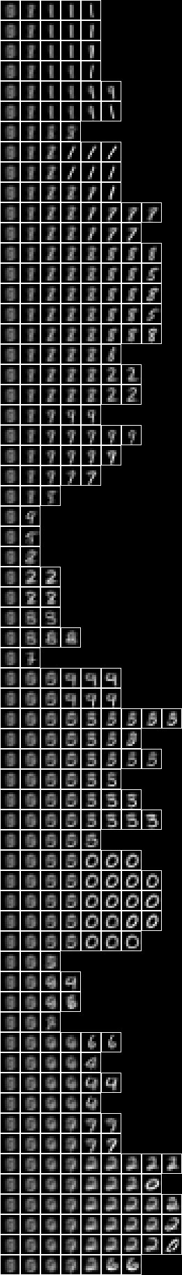
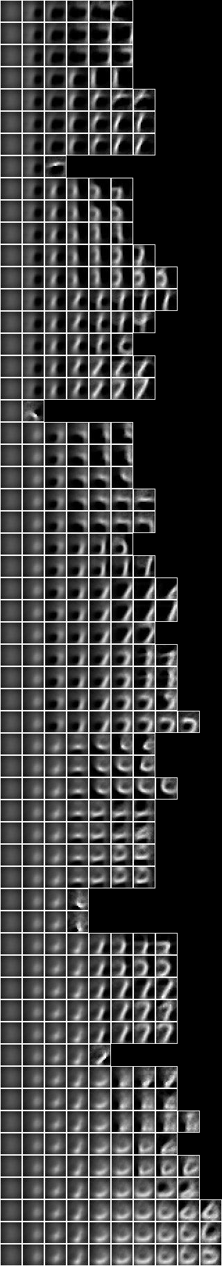
Let us image the fud decomposition,
let file = "NIST.bmp"

bmwrite file $ bmvstack $ map (\bm -> bminsert (bmempty ((28*2)+2) (((28*2)+2)*(maximum (map length pp)))) 0 0 bm) $ map (bmhstack . map (\((_,ff),hrs) -> bmborder 1 (bmmax (hrbm 28 2 2 (hrs `hrhrred` vvk)) 0 0 (hrbm 28 2 2 (qqhr 2 uu vvk (fund ff)))))) pp
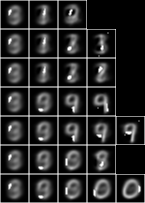
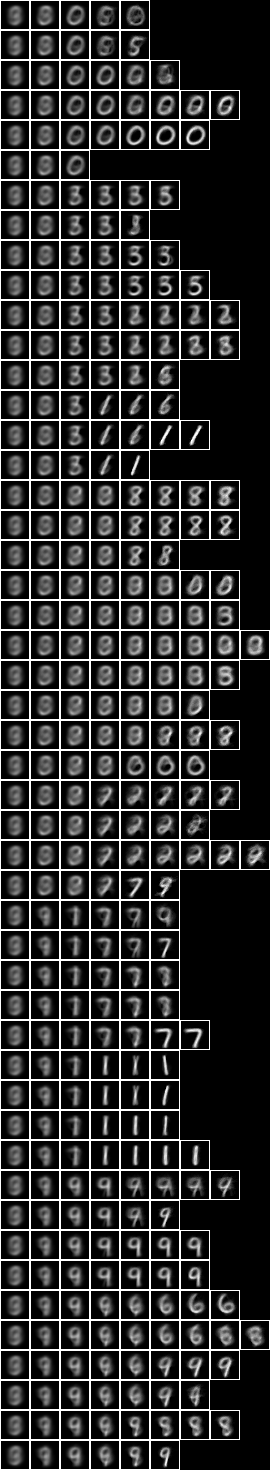
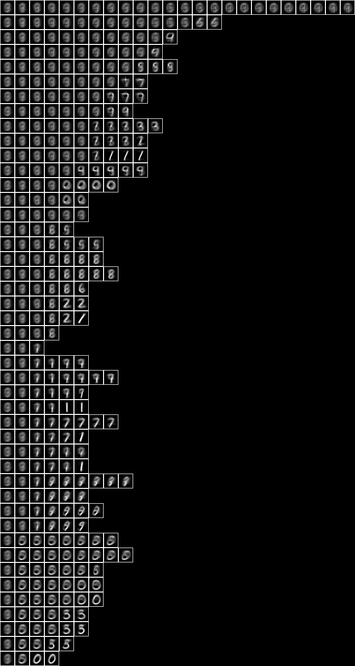
Here we have shown the fud decomposition, $D$, as a vertical stack of decomposition paths of averaged slice images. Each path runs horizontally from the root slice on the left to the leaf slice on the right. The fud underlying variables are also shown superimposed on each slice image. This shows where the ‘attention’ is during decomposition along a path.
The leftmost column contains only the root slice, which is the entire sample of 7500 events. We can also see the root fud underlying variables shown superimposed on the averaged root slice. The underlying tuple here is $\mathrm{und}(F)$, where $((\cdot,F),\cdot) = P_{1,1}$,
let ((_,ff),hrs) = pp !! 0 !! 0

rp $ fund ff
"{<10,10>,<10,11>,<11,9>,<11,10>,<11,11>,<12,9>,<12,10>,<12,11>,<13,9>,<13,10>,<14,9>,<14,10>,<15,9>}"

bmwrite file $ bmborder 1 $ bmmax (hrbm 28 3 2 (hrs `hrhrred` vvk)) 0 0 $ hrbm 28 3 2 $ qqhr 2 uu vvk $ fund ff

It is similar to the first tuple of the investigation of the properties of the sample using the tupler, above.
The second column consists of two children fuds of slice size 2584 and slice size 4513. The first slice is open on the left side of the top loop. It has underlying tuple $\mathrm{und}(F)$, where $((\cdot,F),\cdot) = P_{1,2}$,
let ((_,ff),hrs) = pp !! 0 !! 1

rp $ fund ff
"{<9,16>,<10,16>,<11,15>,<11,16>,<12,15>,<12,16>,<13,15>,<13,16>,<14,14>,<14,15>,<14,16>,<15,15>}"

bmwrite file $ bmborder 1 $ bmmax (hrbm 28 3 2 (hrs `hrhrred` vvk)) 0 0 $ hrbm 28 3 2 $ qqhr 2 uu vvk $ fund ff

The first three rows of the third column consists of two children fuds of slice size 584 and slice size 1295. The first slice looks more like a two than a three now. It has underlying tuple $\mathrm{und}(F)$, where $((\cdot,F),\cdot) = P_{1,3}$,
let ((_,ff),hrs) = pp !! 0 !! 2

rp $ fund ff
"{<10,13>,<10,14>,<11,12>,<11,13>,<11,14>,<12,12>,<12,13>,<13,12>,<13,13>,<14,11>,<14,12>,<14,13>,<15,12>}"

bmwrite file $ bmborder 1 $ bmmax (hrbm 28 3 2 (hrs `hrhrred` vvk)) 0 0 $ hrbm 28 3 2 $ qqhr 2 uu vvk $ fund ff

Following the first row from left to right, we see where the alignments are maximised at each step of the decomposition.
All pixels
Now consider a 127-fud induced model of the 60,000 events of the training sample NIST_model35.json which is induced by NIST_engine35.hs, see Model 35.
We shall analyse it with the 7,500 events subset of the sample,
:l NISTDev

(uu,hrtr) <- nistTrainBucketedIO 2

let digit = VarStr "digit"
let vv = uvars uu
let vvl = sgl digit
let vvk = vv `minus` vvl

let hr = hrev [i | i <- [0.. hrsize hrtr - 1], i `mod` 8 == 0] hrtr

hrsize hr
7500

df <- dfIO "./NIST_model35.json"

let uu1 = uu `uunion` (fsys (dfff df))

card $ dfund df
486

card $ fvars $ dfff df
3929

let (wmax,lmax,xmax,omax,bmax,mmax,umax,pmax,fmax,mult,seed) = (2^11, 8, 2^10, 30, (30*3), 3, 2^8, 1, 127, 1, 5)

summation mult seed uu1 df hr
(129988.66344571306,63698.56389878791)
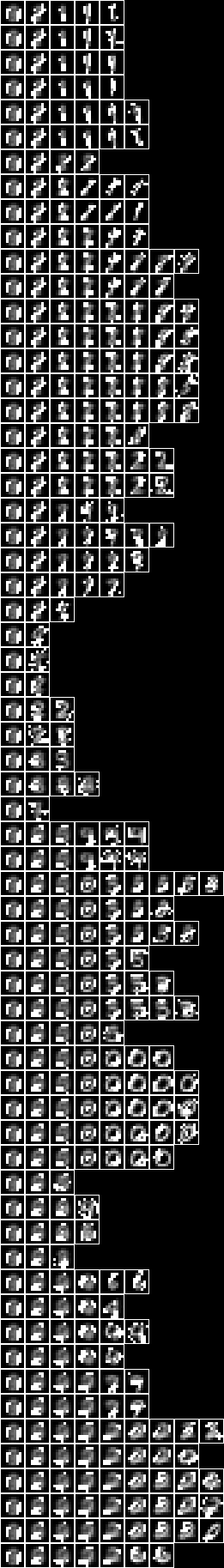
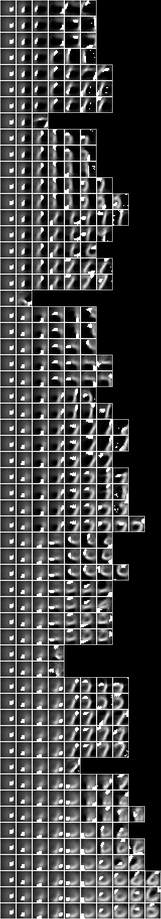
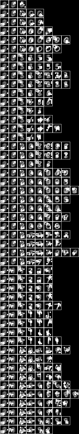
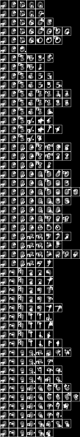
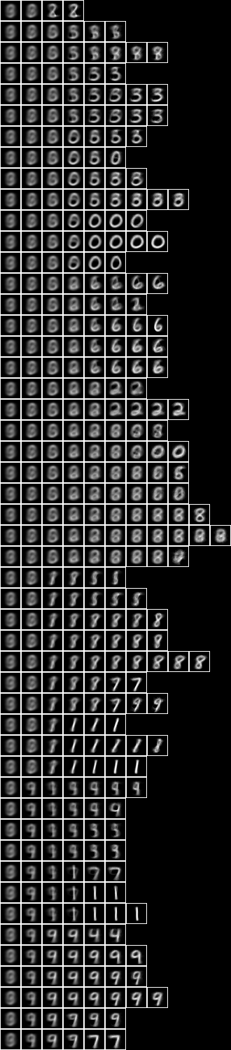
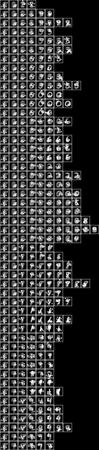
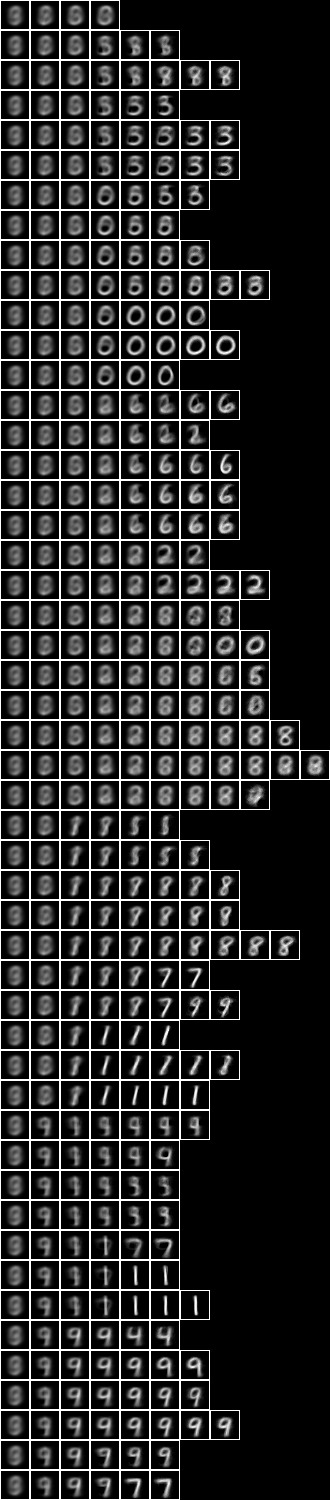
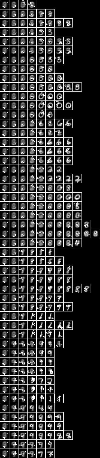
Below is an image of the fud decomposition, and adjacent is an image of the fud underlying superimposed on the slices,
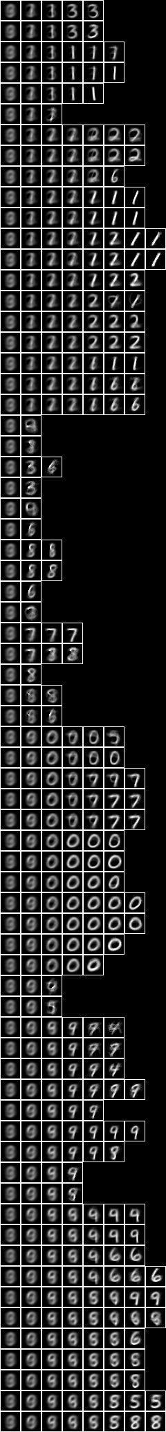
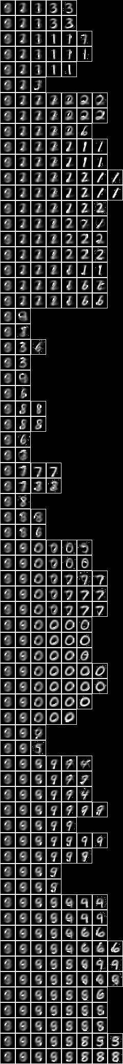
A magnified image of the fud underlying superimposed on the averaged slice, can be seen at Model 35.
Let us analyse the fud decomposition. Let $P = \mathrm{paths}(A * D)$,
let pp = qqll $ treesPaths $ hrmult uu1 df hr

let fid = variablesVariableFud . least . fder

rpln $ map (map (fid . snd . fst)) pp

"[1,3,12,31,104]"
"[1,3,12,31,83]"
"[1,3,12,18,38,72]"
"[1,3,12,18,38,90]"
"[1,3,12,18,54]"
"..."
"[1,92]"
"[1,44,123]"
"[1,44,74]"
"[1,65]"
"[1,113]"
"..."
"[1,2,4,6,8,19,67]"
"[1,2,4,6,8,24,58,127]"
"[1,2,4,6,8,24,59,116]"

rpln $ map (map (hrsize . snd)) pp
"[7500,2259,759,234,103]"
"[7500,2259,759,234,48]"
"[7500,2259,759,460,226,120]"
"[7500,2259,759,460,226,106]"
"[7500,2259,759,460,153]"
"..."
"[7500,68]"
"[7500,144,72]"
"[7500,144,70]"
"[7500,90]"
"[7500,72]"
"..."
"[7500,3568,2078,1394,881,321,111]"
"[7500,3568,2078,1394,881,216,84,40]"
"[7500,3568,2078,1394,881,216,86,59]"
We can see that the paths vary in length from two fuds to eight fuds. The paths of length two have small leaf off-diagonal slices and often seem to contain mixtures of odd cases. Longer paths tend to group more regular and recognisable digits. These paths successively resolve more and more details, such as the obliqueness of ones or the roundness of zeroes. Note that the model does not pay much attention to label alignments. More ‘complicated’ digits, such as fours or fives are neglected in favour of ‘simpler’ digits such as ones and zeroes.
The underlying tuple of the root slice is $\mathrm{und}(F)$, where $((\cdot,F),\cdot) = P_{1,1}$,
let ((_,ff),hrs) = pp !! 0 !! 0

rp $ fund ff
"{<10,11>,<10,12>,<11,10>,<11,11>,<11,12>,<12,9>,<12,10>,<12,11>,<13,9>,<13,10>,<13,11>,<14,9>,<14,10>,<15,9>}"

bmwrite file $ bmborder 1 $ bmmax (hrbm 28 3 2 (hrs `hrhrred` vvk)) 0 0 $ hrbm 28 3 2 $ qqhr 2 uu vvk $ fund ff

It is similar to that of the 15-fud model, above. The first child slice of the second column has size 2259. It resembles the corresponding slice of size 2584 in the 15-fud model. It has quite a different underlying tuple, though,
let ((_,ff),hrs) = pp !! 0 !! 1

rp $ fund ff
"{<18,12>,<18,13>,<19,11>,<19,12>,<19,13>,<20,10>,<20,11>,<20,12>,<20,13>,<21,10>,<21,11>,<21,12>,<21,13>}"

bmwrite file $ bmborder 1 $ bmmax (hrbm 28 3 2 (hrs `hrhrred` vvk)) 0 0 $ hrbm 28 3 2 $ qqhr 2 uu vvk $ fund ff

The 15-fud model 2 resembles the near-root parts of 127-fud model 35. Similarly, varying the parameters of the inducer produces other similar models such as 127-fud model 3 and 127-fud model 4.
Now let us query the model with a sample event to see how it is being classified. First, consider the fud decomposition fud, $F = D^{\mathrm{F}}$, (see Practicable fud decomposition fud),
let ff = dfnul uu1 df 1

card $ fvars $ ff
5483

card $ fder $ ff
1316

rp $ take 20 $ qqll $ fder $ ff
"[<<1,n>,1>,<<1,n>,2>,<<1,n>,3>,<<1,n>,4>,<<1,n>,5>,<<1,n>,6>,<<1,n>,7>,<<1,n>,8>,<<1,n>,9>,<<1,n>,10>,<<1,n>,11>,<<2,n>,1>,<<2,n>,2>,<<2,n>,3>,<<2,n>,4>,<<2,n>,5>,<<2,n>,6>,<<2,n>,7>,<<2,n>,8>,<<2,n>,9>]"
Now apply the model to the sample history, $A_{\mathrm{b}} = A * \prod \mathrm{his}(F)$,
let uu2 = uu `uunion` (fsys ff)

let hrb = hrfmul uu2 ff hr

hrsize hrb
7500

card $ hrvars $ hrb
5782
Choose, for example, the first event $Q = \{S\}^{\mathrm{U}}$, where $S \in (A\%V_{\mathrm{k}})^{\mathrm{S}}$,
let hrq = hrev [0] $ hr `hrhrred` vvk

bmwrite file $ bmborder 1 $ hrbm 28 2 2 $ hrq

Now find the leaf slice of the query, $A_{\mathrm{c}} = A_{\mathrm{b}} * (Q * F^{\mathrm{T}})$,
let hrc = hrhrsel hrb $ hrfmul uu2 ff hrq `hrhrred` fder ff

hrsize hrc
47

bmwrite file $ bmborder 1 $ hrbm 28 2 2 $ hrc `hrhrred` vvk

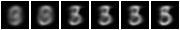
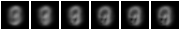
Here are the slice events, $A_{\mathrm{c}}~\%~V_{\mathrm{k}}$,
bmwrite file $ bmhstack $ map (bmborder 1 . hrbm 28 1 2) $ [hrev [i] hr' | let hr' = hrc `hrhrred` vvk, i <- [0..hrsize hrc-1]]

The label variable is, $A_{\mathrm{c}}~\%~V_{\mathrm{l}}$,
rpln $ aall $ hhaa $ hrhh uu1 $ hrc `hrhrred` vvl
"({(digit,0)},2 % 1)"
"({(digit,2)},5 % 1)"
"({(digit,3)},1 % 1)"
"({(digit,4)},3 % 1)"
"({(digit,5)},21 % 1)"
"({(digit,8)},15 % 1)"
The modal label is five, but the slice also contains many eights and some other similar looking digits.
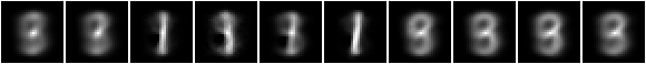
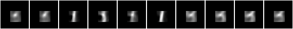
Now let us see how the slice was chosen. Here are the slices and their underlying for each non-null derived variable state, \[ \{A_{\mathrm{b}} * \{\{(w,u)\}\}^{\mathrm{U}}~\%~\{w\} : (S,\cdot) \in A_{\mathrm{c}}~\%~\mathrm{der}(F),~(w,u) \in S,~u \neq \mathrm{null}\} \]
let ll = [(w,u) | (ss,_) <- (aall $ hhaa $ hrhh uu2 $ hrc `hrhrred` fder ff), (w,u) <- ssll ss, u /= ValStr("null")]

rpln [hhaa (hrhh uu2 (hrb' `hrhrsel` aahr uu2 rr `hrhrred` (vars rr))) | let hrb' = hrb `hrhrred` (vvk `union` llqq (map fst ll)),  (w,u) <- ll, let rr = single (llss [(w,u)]) 1]
"{({(<<1,n>,1>,1)},4662 % 1)}"
"{({(<<1,n>,2>,0)},3325 % 1)}"
"{({(<<1,n>,3>,0)},2814 % 1)}"
"{({(<<1,n>,4>,0)},2943 % 1)}"
"{({(<<1,n>,5>,0)},3021 % 1)}"
"{({(<<1,n>,6>,0)},3435 % 1)}"
"{({(<<1,n>,7>,1)},4651 % 1)}"
"{({(<<1,n>,8>,0)},3215 % 1)}"
"{({(<<1,n>,9>,1)},4726 % 1)}"
"{({(<<1,n>,10>,0)},3255 % 1)}"
"{({(<<1,n>,11>,0)},3040 % 1)}"
"{({(<<44,n>,1>,1)},71 % 1)}"
"{({(<<44,n>,2>,1)},71 % 1)}"
"{({(<<44,n>,3>,1)},72 % 1)}"
"{({(<<44,n>,4>,1)},71 % 1)}"
"{({(<<44,n>,5>,1)},72 % 1)}"
"{({(<<44,n>,6>,1)},72 % 1)}"
"{({(<<44,n>,7>,1)},71 % 1)}"
"{({(<<44,n>,8>,1)},71 % 1)}"
"{({(<<44,n>,9>,1)},72 % 1)}"
"{({(<<44,n>,10>,1)},71 % 1)}"
"{({(<<44,n>,11>,1)},71 % 1)}"
"{({(<<74,n>,1>,1)},47 % 1)}"
"{({(<<74,n>,2>,1)},47 % 1)}"
"{({(<<74,n>,3>,1)},47 % 1)}"
"{({(<<74,n>,4>,1)},47 % 1)}"
"{({(<<74,n>,5>,1)},47 % 1)}"
"{({(<<74,n>,6>,1)},47 % 1)}"
"{({(<<74,n>,7>,1)},47 % 1)}"
"{({(<<74,n>,8>,1)},47 % 1)}"
"{({(<<74,n>,9>,1)},47 % 1)}"
"{({(<<74,n>,10>,1)},47 % 1)}"
"{({(<<74,n>,11>,1)},47 % 1)}"

bmwrite file $ bmhstack $ map (bmborder 1 . hrbm 28 1 2) $ [hrb' `hrhrsel` aahr uu2 rr `hrhrred` vvk | let hrb' = hrb `hrhrred` (vvk `union` llqq (map fst ll)),  (w,u) <- ll, let rr = single (llss [(w,u)]) 1]

bmwrite file $ bmhstack $ map (bmborder 1 . hrbm 28 1 2) $ [qqhr 2 uu vvk (fund (ff `fdep` sgl w)) | (w,u) <- ll, let rr = single (llss [(w,u)]) 1]


In this case, we can see that there are only three fuds in the decomposition path, with little to distinguish between the derived variables of the last two fuds.
Now let us repeat the same analysis for the next event,
let hrq = hrev [1] $ hr `hrhrred` vvk

bmwrite file $ bmborder 1 $ hrbm 28 2 2 $ hrq

Now find the leaf slice of the query,
let hrc = hrhrsel hrb $ hrfmul uu2 ff hrq `hrhrred` fder ff

hrsize hrc
50

bmwrite file $ bmborder 1 $ hrbm 28 2 2 $ hrc `hrhrred` vvk

Here are the slice events,
bmwrite file $ bmhstack $ map (bmborder 1 . hrbm 28 1 2) $ [hrev [i] hr' | let hr' = hrc `hrhrred` vvk, i <- [0..hrsize hrc-1]]

The label variable is,
rpln $ aall $ hhaa $ hrhh uu1 $ hrc `hrhrred` vvl
"({(digit,1)},50 % 1)"
In this case the entire slice consists of ones.
Here are the slices and their underlying for each non-null derived variable state,
let ll = [(w,u) | (ss,_) <- (aall $ hhaa $ hrhh uu2 $ hrc `hrhrred` fder ff), (w,u) <- ssll ss, u /= ValStr("null")]

rpln [hhaa (hrhh uu2 (hrb' `hrhrsel` aahr uu2 rr `hrhrred` (vars rr))) | let hrb' = hrb `hrhrred` (vvk `union` llqq (map fst ll)),  (w,u) <- ll, let rr = single (llss [(w,u)]) 1]
"{({(<<1,n>,1>,0)},2838 % 1)}"
"{({(<<1,n>,2>,0)},3325 % 1)}"
"{({(<<1,n>,3>,0)},2814 % 1)}"
"{({(<<1,n>,4>,0)},2943 % 1)}"
"{({(<<1,n>,5>,0)},3021 % 1)}"
"{({(<<1,n>,6>,0)},3435 % 1)}"
"{({(<<1,n>,7>,0)},2849 % 1)}"
"{({(<<1,n>,8>,0)},3215 % 1)}"
"{({(<<1,n>,9>,0)},2774 % 1)}"
"{({(<<1,n>,10>,0)},3255 % 1)}"
"{({(<<1,n>,11>,0)},3040 % 1)}"
"{({(<<3,n>,1>,0)},1034 % 1)}"
"{({(<<3,n>,2>,0)},919 % 1)}"
"{({(<<3,n>,3>,0)},966 % 1)}"
"{({(<<3,n>,4>,0)},940 % 1)}"
"{({(<<3,n>,5>,0)},909 % 1)}"
"{({(<<3,n>,6>,0)},975 % 1)}"
"{({(<<3,n>,7>,0)},917 % 1)}"
"{({(<<3,n>,8>,0)},914 % 1)}"
"{({(<<3,n>,9>,0)},965 % 1)}"
"{({(<<3,n>,10>,0)},1002 % 1)}"
"{({(<<3,n>,11>,0)},894 % 1)}"
"{({(<<12,n>,1>,1)},510 % 1)}"
"{({(<<12,n>,2>,1)},512 % 1)}"
"{({(<<12,n>,3>,1)},465 % 1)}"
"{({(<<12,n>,4>,1)},485 % 1)}"
"{({(<<12,n>,5>,1)},510 % 1)}"
"{({(<<12,n>,6>,1)},494 % 1)}"
"{({(<<12,n>,7>,1)},500 % 1)}"
"{({(<<12,n>,8>,1)},493 % 1)}"
"{({(<<12,n>,9>,1)},492 % 1)}"
"{({(<<12,n>,10>,1)},498 % 1)}"
"{({(<<12,n>,11>,1)},504 % 1)}"
"{({(<<18,n>,1>,1)},212 % 1)}"
"{({(<<18,n>,2>,1)},179 % 1)}"
"{({(<<18,n>,3>,1)},204 % 1)}"
"{({(<<18,n>,4>,1)},177 % 1)}"
"{({(<<18,n>,5>,1)},168 % 1)}"
"{({(<<18,n>,6>,1)},183 % 1)}"
"{({(<<18,n>,7>,1)},192 % 1)}"
"{({(<<18,n>,8>,1)},192 % 1)}"
"{({(<<18,n>,9>,1)},184 % 1)}"
"{({(<<18,n>,10>,1)},203 % 1)}"
"{({(<<18,n>,11>,1)},198 % 1)}"
"{({(<<54,n>,1>,0)},94 % 1)}"
"{({(<<54,n>,2>,1)},75 % 1)}"
"{({(<<54,n>,3>,1)},75 % 1)}"
"{({(<<54,n>,4>,1)},75 % 1)}"
"{({(<<54,n>,5>,2)},75 % 1)}"
"{({(<<54,n>,6>,1)},75 % 1)}"
"{({(<<54,n>,7>,1)},74 % 1)}"

bmwrite file $ bmhstack $ map (bmborder 1 . hrbm 28 1 2) $ [hrb' `hrhrsel` aahr uu2 rr `hrhrred` vvk | let hrb' = hrb `hrhrred` (vvk `union` llqq (map fst ll)),  (w,u) <- ll, let rr = single (llss [(w,u)]) 1]

bmwrite file $ bmhstack $ map (bmborder 1 . hrbm 28 1 2) $ [qqhr 2 uu vvk (fund (ff `fdep` sgl w)) | (w,u) <- ll, let rr = single (llss [(w,u)]) 1]


Now there are five fuds in the decomposition path, so the classification is more gradual.
Averaged pixels
Now consider a 127-fud induced model of the 60,000 events of the training sample NIST_model34.json which is induced by NIST_engine34.hs, (see Model 34).
We shall analyse it with the 7,500 events subset of the sample,
:l NISTDev

(uu,hrtr) <- nistTrainBucketedAveragedIO 8 9 0

let digit = VarStr "digit"
let vv = uvars uu
let vvl = sgl digit
let vvk = vv `minus` vvl

let hr = hrev [i | i <- [0.. hrsize hrtr - 1], i `mod` 8 == 0] hrtr

hrsize hr
7500

df <- dfIO "./NIST_model34.json"

let uu1 = uu `uunion` (fsys (dfff df))

card $ dfund df
70

card $ fvars $ dfff df
4811

let (wmax,lmax,xmax,omax,bmax,mmax,umax,pmax,fmax,mult,seed) = (2^11, 8, 2^10, 30, (30*3), 3, 2^8, 1, 127, 1, 5)

summation mult seed uu1 df hr
(89445.55032765196,43702.20275253874)
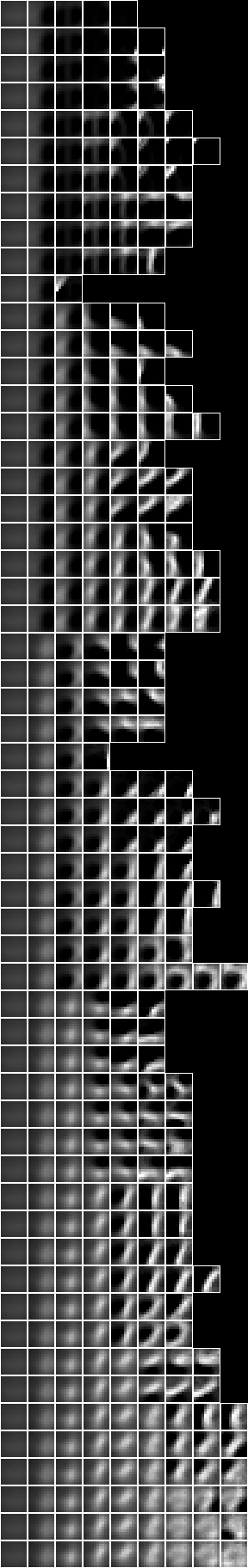
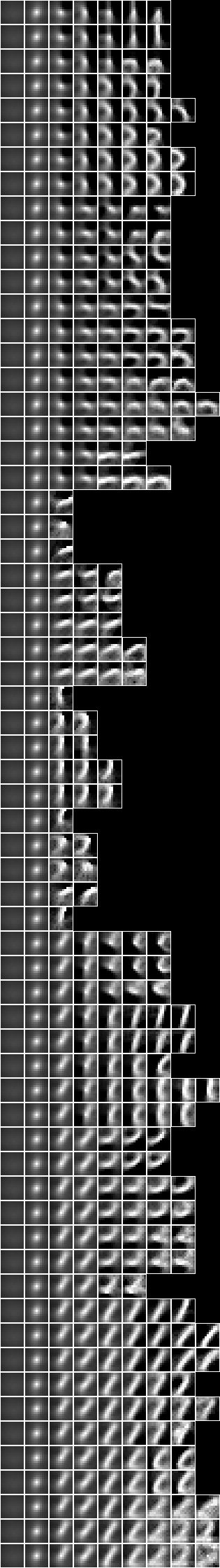
Below is an image of the fud decomposition, and adjacent is an image of the fud underlying superimposed on the slices,
A magnified image of the fud underlying superimposed on the averaged slice, can be seen at Model 34.
let pp = qqll $ treesPaths $ hrmult uu1 df hr

rpln $ map (map (hrsize . snd)) pp
"[7500,2500,773,373,94]"
"[7500,2500,773,373,72]"
"[7500,2500,773,373,68]"
"..."
"[7500,2500,596,126,68]"
"[7500,2500,80]"
"[7500,41]"
"[7500,9]"
"[7500,40]"
"[7500,61,27]"
"[7500,56,49]"
"[7500,120,55]"
"[7500,120,63,37]"
"[7500,51]"
"[7500,4259,2045,509,176,63]"
"..."
"[7500,4259,1674,462,208,161,74,53,9]"
"[7500,4259,1674,462,208,161,74,19,2]"
"[7500,4259,1674,462,208,47,28]"
Similarly to the all-pixels case above, we can see that the paths vary in length from two fuds to nine fuds. Here the clusters of the underlying tuples are spread over more of the digit, and so the classification is less localised. The longer paths divide less according to style and more according to label, than the all-pixels model.
The underlying tuple of the root slice is,
let ((_,ff),hrs) = pp !! 0 !! 0

rp $ fund ff
"{<4,3>,<4,4>,<4,8>,<5,3>,<5,7>,<5,8>,<6,3>,<6,7>,<6,8>,<7,3>,<7,7>,<7,8>,<8,7>}"

bmwrite file $ bmborder 1 $ bmmax (hrbm 9 (3*2) 8 (hrs `hrhrred` vvk)) 0 0 $ hrbm 9 (3*2) 8 $ qqhr 8 uu vvk $ fund ff

It is similar to the first tuple of the investigation of the properties of the sample using the tupler, above.
Square regions of 10x10 pixels
Now consider a 127-fud induced model of square regions of 10x10 pixels chosen randomly from the images of the 60,000 events of the training sample NIST_model6.json which is induced by NIST_engine6.hs. (See Model induction.)
We shall analyse it with the 7,500 events subset of the sample,
:l NISTDev

(uu,hrtr) <- nistTrainBucketedRegionRandomIO 2 10 17

let digit = VarStr "digit"
let vv = uvars uu
let vvl = sgl digit
let vvk = vv `minus` vvl

let hr = hrev [i | i <- [0.. hrsize hrtr - 1], i `mod` 8 == 0] hrtr

hrsize hr
7500

df <- dfIO "./NIST_model6.json"

let uu1 = uu `uunion` (fsys (dfff df))

card $ dfund df
100

card $ fvars $ dfff df
3659

let (wmax,lmax,xmax,omax,bmax,mmax,umax,pmax,fmax,mult,seed) = (2^11, 8, 2^10, 30, (30*3), 3, 2^8, 1, 127, 1, 5)

summation mult seed uu1 df hr
(184576.57927767973,91637.00512528208)
Imaging the fud decomposition,
Square regions of 15x15 pixels
Now consider a 127-fud induced model of square regions of 15x15 pixels chosen randomly from the images of the 60,000 events of the training sample NIST_model21.json which is induced by NIST_engine21.hs. (See Model induction.)
We shall analyse it with the 7,500 events subset of the sample,
:l NISTDev

(uu,hrtr) <- nistTrainBucketedRegionRandomIO 2 15 17

let digit = VarStr "digit"
let vv = uvars uu
let vvl = sgl digit
let vvk = vv `minus` vvl

let hr = hrev [i | i <- [0.. hrsize hrtr - 1], i `mod` 8 == 0] hrtr

hrsize hr
7500

df <- dfIO "./NIST_model21.json"

let uu1 = uu `uunion` (fsys (dfff df))

card $ dfund df
225

card $ fvars $ dfff df
4086

let (wmax,lmax,xmax,omax,bmax,mmax,umax,pmax,fmax,mult,seed) = (2^11, 8, 2^10, 30, (30*3), 3, 2^8, 1, 127, 1, 5)

summation mult seed uu1 df hr
(175450.03386620025,87200.2600512719)
Imaging the fud decomposition,
Centred square regions of 11x11 pixels
Now consider a 127-fud induced model applied to centred square regions of 11x11 pixels chosen randomly from the images of the 60,000 events of the training sample NIST_model10.json which is induced by NIST_engine10.hs. (See Model induction.)
We shall analyse it with the 7,500 events subset of the sample,
:l NISTDev

(uu,hrtr) <- nistTrainBucketedRegionRandomIO 2 11 17

let digit = VarStr "digit"
let vv = uvars uu
let vvl = sgl digit
let vvk = vv `minus` vvl

let hr = hrev [i | i <- [0.. hrsize hrtr - 1], i `mod` 8 == 0] hrtr

hrsize hr
7500

df <- dfIO "./NIST_model10.json"

let uu1 = uu `uunion` (fsys (dfff df))

card $ dfund df
121

card $ fvars $ dfff df
3975

let (wmax,lmax,xmax,omax,bmax,mmax,umax,pmax,fmax,mult,seed) = (2^11, 8, 2^10, 30, (30*3), 3, 2^8, 1, 127, 1, 5)

summation mult seed uu1 df hr
(29422.851711477848,14570.720140287482)
Imaging the fud decomposition,

Row and column regions
Now consider a 127-fud induced model applied to row regions of 1x28 pixels chosen randomly from the images of the 60,000 events of the training sample NIST_model18_rows.json which is induced by NIST_engine18.hs. (See Model induction.)
We shall analyse it with the 7,500 events subset of the sample,
:l NISTDev

(uu,hrtr) <- nistTrainBucketedRectangleRandomIO 2 1 28 17

let digit = VarStr "digit"
let vv = uvars uu
let vvl = sgl digit
let vvk = vv `minus` vvl

let hr = hrev [i | i <- [0.. hrsize hrtr - 1], i `mod` 8 == 0] hrtr

hrsize hr
7500

df <- dfIO "./NIST_model18_rows.json"

let uu1 = uu `uunion` (fsys (dfff df))

card $ dfund df
26

card $ fvars $ dfff df
2030

let (wmax,lmax,xmax,omax,bmax,mmax,umax,pmax,fmax,mult,seed) = (2^11, 8, 2^10, 30, (30*3), 3, 2^8, 1, 127, 1, 5)

summation mult seed uu1 df hr
(89543.73634504592,43118.82498986515)
This summed alignment is considerably lower than for square regions, because of the smaller substrate.
Again, consider a 127-fud induced model applied to column regions of 28x1 pixels chosen randomly from the images of the 60,000 events of the training sample NIST_model18_cols.json which is induced by NIST_engine18.hs. (See Model induction.)
We shall analyse it with the 7,500 events subset of the sample,
:l NISTDev

(uu,hrtr) <- nistTrainBucketedRectangleRandomIO 2 28 1 17

let digit = VarStr "digit"
let vv = uvars uu
let vvl = sgl digit
let vvk = vv `minus` vvl

let hr = hrev [i | i <- [0.. hrsize hrtr - 1], i `mod` 8 == 0] hrtr

hrsize hr
7500

df <- dfIO "./NIST_model18_cols.json"

let uu1 = uu `uunion` (fsys (dfff df))

card $ dfund df
27

card $ fvars $ dfff df
2953

let (wmax,lmax,xmax,omax,bmax,mmax,umax,pmax,fmax,mult,seed) = (2^11, 8, 2^10, 30, (30*3), 3, 2^8, 1, 127, 1, 5)

summation mult seed uu1 df hr
(73799.87428828268,34870.49167826719)
Again, this summed alignment is considerably lower than for square regions, because of the smaller substrate.
Two level over 10x10 regions
Let us consider a two level model which consists of 5x5 frames of square regions of 10x10 pixels.
First we will reduce the underlying 127-fud decomposition $D$ so that the resultant decomposition fud does not make an excessively large level substrate. The reduced decomposition is a sub-model constructed by selecting only one derived variable and its dependents in each fud of the decomposition. In the case where the fuds are highly diagonalised this usually leads to a reasonable approximation of the model. Let us examine this reduced decomposition $D_{\mathrm{r}}$,
:l NISTDev

(uu,hrtr) <- nistTrainBucketedRegionRandomIO 2 10 17

let digit = VarStr "digit"
let vv = uvars uu
let vvl = sgl digit
let vvk = vv `minus` vvl

let hr = hrev [i | i <- [0.. hrsize hrtr - 1], i `mod` 8 == 0] hrtr

hrsize hr
7500

df <- dfIO "./NIST_model6.json"

let uu1 = uu `uunion` (fsys (dfff df))

card $ dfund df
100

card $ fder $ dfff df
1302

card $ fvars $ dfff df
3659

let dfred = systemsDecompFudsHistoryRepasDecompFudReduced

let dfr = dfred uu1 df hr

card $ dfund dfr
100

card $ fder $ dfff dfr
126

card $ fvars $ dfff dfr
567
Imaging the reduced fud decomposition,
let pp = qqll $ treesPaths $ hrmult uu1 dfr hr

bmwrite file $ bmvstack $ map (\bm -> bminsert (bmempty ((10*3)+2) (((10*3)+2)*(maximum (map length pp)))) 0 0 bm) $ map (bmhstack . map (\(_,hrs) -> bmborder 1 (hrbm 10 3 2 (hrs `hrhrred` vvk)))) $ pp
The reduced fud decomposition on the left may be compared to the original fud decomposition on the right,

The images are similar in spite of the reduction.
Having reduced the level 1 model we can then make 5x5 copies of it to cover the 28x28 pixels of the sample substrate - see Model induction. The model NIST_model24.json is induced by NIST_engine24.hs.
We shall analyse it with the 7,500 events subset of the sample,
:l NISTDev

(uu,hrtr) <- nistTrainBucketedIO 2

let digit = VarStr "digit"
let vv = uvars uu
let vvl = sgl digit
let vvk = vv `minus` vvl

let hr = hrev [i | i <- [0.. hrsize hrtr - 1], i `mod` 8 == 0] hrtr

hrsize hr
7500

df <- dfIO "./NIST_model24.json"

let uu1 = uu `uunion` (fsys (dfff df))

card $ dfund df
642

card $ fder $ dfff df
1321

card $ fvars $ dfff df
6158

let (wmax,lmax,xmax,omax,bmax,mmax,umax,pmax,fmax,mult,seed) = (2^11, 8, 2^10, 30, (30*3), 3, 2^8, 1, 127, 1, 5)

summation mult seed uu1 df hr
(197806.77675500445,94133.42748410173)
We can compare this 2-level model to the all pixels 1-level model,
summation mult seed uu1 df hr
(129988.66344571306,63698.56389878791)
The 2-level model is considerably more aligned.
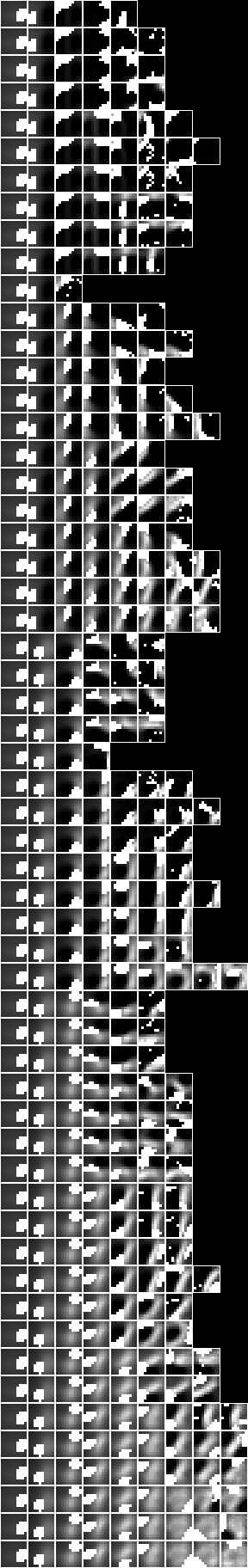
Below is an image of the fud decomposition, and adjacent is an image of the fud underlying superimposed on the slices,
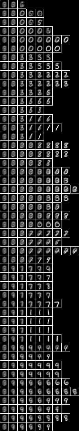
A magnified image of the fud underlying superimposed on the averaged slice, can be seen at Model 24.
We can see that the fud underlying clusters are larger in general than for the 1-level model. The paths vary in length from three fuds to eight fuds. The tree is more uniform than for the 1-level model. That is, there are fewer effective off-diagonal states.
Let us reduce the 2-level model, $D$, to make it more managable, $D_{\mathrm{r}}$,
let dfr = dfred uu1 df hr

card $ dfund dfr
627

card $ fder $ dfff dfr
127

card $ fvars $ dfff dfr
3598
Let us examine the slices, $P = \mathrm{paths}(A * D_{\mathrm{r}})$,
let pp = qqll $ treesPaths $ hrmult uu1 dfr hr

let variablesVariableFud (VarPair (VarPair (VarPair (f,_),_),_)) = f
    variablesVariableFud _ = VarInt 0

let fid = variablesVariableFud . least . fder

rpln $ zip [0..] $ map (map (fid . snd . fst)) pp
"(0,[1,2,13,50,104])"
"(1,[1,2,13,50,95])"
"(2,[1,2,13,19,30,126])"
"..."
"(6,[1,2,7,38,62,112])"
"..."
"(11,[1,2,7,14,23,33,59,101])"
"..."
"(35,[1,3,8,18,43,105])"
"..."
"(46,[1,3,6,10,16,40,113])"
"(47,[1,3,6,10,32,54,76,122])"
"(48,[1,3,6,10,32,99])"

rpln $ zip [0..] $ map (map (hrsize . snd)) pp
"(0,[7500,3857,888,249,129])"
"(1,[7500,3857,888,249,120])"
"(2,[7500,3857,888,639,368,164])"
"..."
"(6,[7500,3857,1177,1047,930,443])"
"..."
"(11,[7500,3857,1177,1047,607,521,221,118])"
"..."
"(35,[7500,3643,1623,775,346,167])"
"..."
"(46,[7500,3643,2020,1082,716,228,93])"
"(47,[7500,3643,2020,1082,366,250,181,136])"
"(48,[7500,3643,2020,1082,366,116])"
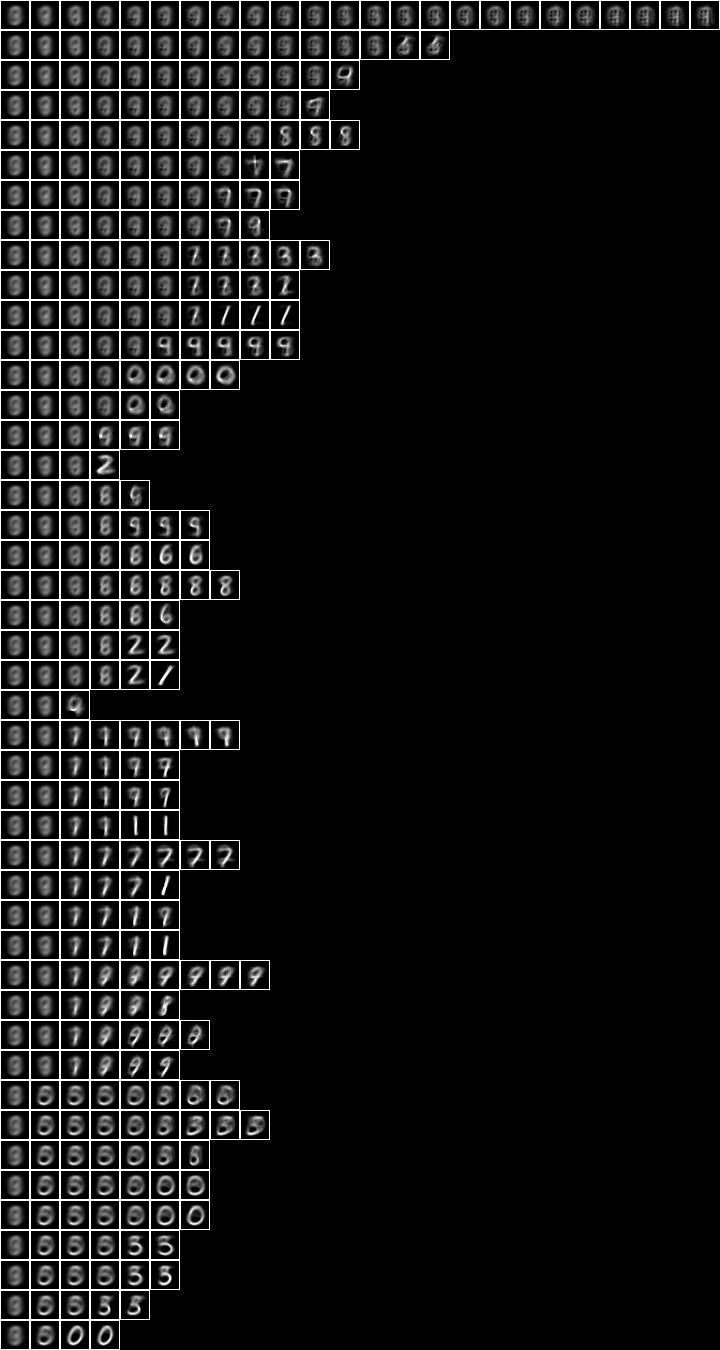
Imaging the reduced decomposition slices,
bmwrite file $ bmvstack $ map (\bm -> bminsert (bmempty (28+2) ((28+2)*(maximum (map length pp)))) 0 0 bm) $ map (bmhstack . map (\(_,hrs) -> bmborder 1 (hrbm 28 1 2 (hrs `hrhrred` vvk)))) pp

bmwrite file $ bmvstack $ map (\bm -> bminsert (bmempty (28+2) ((28+2)*(maximum (map length pp)))) 0 0 bm) $ map (bmhstack . map (\((_,ff),hrs) -> bmborder 1 (bmmax (hrbm 28 1 2 (hrs `hrhrred` vvk)) 0 0 (hrbm 28 1 2 (qqhr 2 uu vvk (fund ff)))))) pp
Again, the reduced decomposition is similar to the original decomposition.
The underlying tuple of the root slice is $\mathrm{und}(F)$, where $((\cdot,F),\cdot) = P_{1,1}$,
let ((_,ff),hrs) = pp !! 0 !! 0

card $ fund ff
91

bmwrite file $ bmborder 1 $ bmmax (hrbm 28 3 2 (hrs `hrhrred` vvk)) 0 0 $ hrbm 28 3 2 $ qqhr 2 uu vvk $ fund ff

We can see that the root slice depends on an underlying cluster that is larger than the corresponding cluster for the root slice in the 1-level model. It is also in a different location.
The first child slice of the second column has size 3857,
let ((_,ff),hrs) = pp !! 0 !! 1

card $ fund ff
52

bmwrite file $ bmborder 1 $ bmmax (hrbm 28 3 2 (hrs `hrhrred` vvk)) 0 0 $ hrbm 28 3 2 $ qqhr 2 uu vvk $ fund ff

Again, we can see that the root slice depends on a larger cluster of the substrate than in the 1-level model.
Now let us query the model with a sample event to see how it is being classified. First, consider the fud decomposition fud, $F = D_{\mathrm{r}}^{\mathrm{F}}$, (see Practicable fud decomposition fud),
let ff = dfnul uu1 dfr 2

card $ fvars $ ff
3975

card $ fder $ ff
127

rp $ take 5 $ qqll $ fder $ ff
"[<<<1,1>,n2>,1>,<<<2,1>,n2>,1>,<<<3,1>,n2>,1>,<<<4,1>,n2>,1>,<<<5,1>,n2>,1>]"
Now apply the model to the sample history, $A_{\mathrm{b}} = A * \prod \mathrm{his}(F)$,
let uu2 = uu `uunion` (fsys ff)

let hrb = hrfmul uu2 ff hr

hrsize hrb
7500

card $ hrvars $ hrb
4133
Choose, for example, the first event $Q = \{S\}^{\mathrm{U}}$, where $S \in (A\%V_{\mathrm{k}})^{\mathrm{S}}$,
let hrq = hrev [0] $ hr `hrhrred` vvk

bmwrite file $ bmborder 1 $ hrbm 28 2 2 $ hrq
Now find the leaf slice of the query, $A_{\mathrm{c}} = A_{\mathrm{b}} * (Q * F^{\mathrm{T}})$,
let hrc = hrhrsel hrb $ hrfmul uu2 ff hrq `hrhrred` fder ff

hrsize hrc
10

bmwrite file $ bmborder 1 $ hrbm 28 2 2 $ hrc `hrhrred` vvk

Here are the slice events, $A_{\mathrm{c}}~\%~V_{\mathrm{k}}$,
bmwrite file $ bmhstack $ map (bmborder 1 . hrbm 28 1 2) $ [hrev [i] hr' | let hr' = hrc `hrhrred` vvk, i <- [0..hrsize hrc-1]]

The label variable is, $A_{\mathrm{c}}~\%~V_{\mathrm{l}}$,
rpln $ aall $ hhaa $ hrhh uu1 $ hrc `hrhrred` vvl
"({(digit,5)},6 % 1)"
"({(digit,6)},2 % 1)"
"({(digit,7)},1 % 1)"
"({(digit,8)},1 % 1)"
The modal label is five, but the slice has some other similar looking digits.
Now let us see how the event was chosen. Here are the slices and their underlying for each non-null derived variable state, \[ \{A_{\mathrm{b}} * \{\{(w,u)\}\}^{\mathrm{U}}~\%~\{w\} : (S,\cdot) \in Q * F^{\mathrm{T}},~(w,u) \in S,~u \neq \mathrm{null}\} \]
let hrqb = hrfmul uu2 ff hrq

let ll = [(w,u) | (ss,_) <- (aall $ hhaa $ hrhh uu2 $ hrqb `hrhrred` fder ff), (w,u) <- ssll ss, u /= ValStr("null")]

rpln [hhaa (hrhh uu2 (hrb' `hrhrsel` aahr uu2 rr `hrhrred` (vars rr))) | let hrb' = hrb `hrhrred` (vvk `union` llqq (map fst ll)),  (w,u) <- ll, let rr = single (llss [(w,u)]) 1]
"{({(<<<1,1>,n2>,1>,0)},3857 % 1)}"
"{({(<<<2,1>,n2>,1>,1)},1177 % 1)}"
"{({(<<<7,1>,n2>,1>,0)},1047 % 1)}"
"{({(<<<14,1>,n2>,1>,1)},607 % 1)}"
"{({(<<<23,1>,n2>,1>,0)},521 % 1)}"
"{({(<<<33,1>,n2>,1>,1)},221 % 1)}"
"{({(<<<38,1>,n2>,1>,0)},930 % 1)}"
"{({(<<<59,1>,n2>,1>,1)},118 % 1)}"
"{({(<<<62,1>,n2>,1>,1)},443 % 1)}"
"{({(<<<101,1>,n2>,1>,0)},32 % 1)}"
"{({(<<<112,1>,n2>,1>,1)},180 % 1)}"

bmwrite file $ bmhstack $ map (bmborder 1 . hrbm 28 2 2) $ [hrb' `hrhrsel` aahr uu2 rr `hrhrred` vvk | let hrb' = hrb `hrhrred` (vvk `union` llqq (map fst ll)),  (w,u) <- ll, let rr = single (llss [(w,u)]) 1]

bmwrite file $ bmhstack $ map (bmborder 1 . hrbm 28 2 2) $ [qqhr 2 uu vvk (fund (ff `fdep` sgl w)) | (w,u) <- ll, let rr = single (llss [(w,u)]) 1]


Note that we are considering the reduced decomposition, $D_{\mathrm{r}}$, which can be indistinct, so the non-null derived variables do not necessarily correspond to just one path of the original decomposition, $D$. In this case they correspond to two paths,
"..."
"(6,[1,2,7,38,62,112])"
"..."
"(11,[1,2,7,14,23,33,59,101])"
"..."

bmwrite file $ bmhstack $ map (\(_,hrs) -> bmborder 1 (hrbm 28 1 2 (hrs `hrhrred` vvk))) $ pp !! 6

bmwrite file $ bmhstack $ map (\(_,hrs) -> bmborder 1 (hrbm 28 1 2 (hrs `hrhrred` vvk))) $ pp !! 11
The leaf derived variables, <<<101,1>,n2>,1> and <<<112,1>,n2>,1>, cover large parts of the substrate.
Let us examine the level 1 nullable derived variables of the central region at (10;10),
let islevnull (VarPair (VarPair (VarPair (_, VarStr "n"), _), VarStr "(10;10)")) = True
    islevnull _ = False

card $ Set.filter islevnull $ fvars $ ff
12

let ll = qqll $ llqq [(w,u) | (ss,_) <- (aall $ hhaa $ hrhh uu2 $ hrqb `hrhrred` Set.filter islevnull (fvars ff)), (w,u) <- ssll ss, u /= ValStr("null")]

rpln [hhaa (hrhh uu2 (hrb' `hrhrsel` aahr uu2 rr `hrhrred` (vars rr))) | let hrb' = hrb `hrhrred` (vvk `union` llqq (map fst ll)),  (w,u) <- ll, let rr = single (llss [(w,u)]) 1]
"{({(<<<<<1,1>,0>,n>,1>,(10;10)>,1)},6642 % 1)}"
"{({(<<<<<1,2>,0>,n>,1>,(10;10)>,1)},5560 % 1)}"

bmwrite file $ bmhstack $ map (bmborder 1 . hrbm 28 2 2) $ [hrb' `hrhrsel` aahr uu2 rr `hrhrred` vvk | let hrb' = hrb `hrhrred` (vvk `union` llqq (map fst ll)),  (w,u) <- ll, let rr = single (llss [(w,u)]) 1]

let bmmask = bminsert (bmempty (28*2) (28*2)) (((28-10-10)*2)-1) ((10*2)-1) (bmfull (10*2) (10*2))

bmwrite file $ bmhstack $ map (bmborder 1 . bmmin bmmask 0 0 . hrbm 28 2 2) $ [hrb' `hrhrsel` aahr uu2 rr `hrhrred` vvk | let hrb' = hrb `hrhrred` (vvk `union` llqq (map fst ll)),  (w,u) <- ll, let rr = single (llss [(w,u)]) 1]

bmwrite file $ bmhstack $ map (bmborder 1 . hrbm 28 2 2) $ [qqhr 2 uu vvk (fund (ff `fdep` sgl w)) | (w,u) <- ll, let rr = single (llss [(w,u)]) 1]

This frame detects the middle section of the five.
We can compare this region to the region, say, at (2;18),
let islevnull (VarPair (VarPair (VarPair (_, VarStr "n"), _), VarStr "(2;18)")) = True
    islevnull _ = False

card $ Set.filter islevnull $ fvars $ ff
9

let ll = qqll $ llqq [(w,u) | (ss,_) <- (aall $ hhaa $ hrhh uu2 $ hrqb `hrhrred` Set.filter islevnull (fvars ff)), (w,u) <- ssll ss, u /= ValStr("null")]

rpln [hhaa (hrhh uu2 (hrb' `hrhrsel` aahr uu2 rr `hrhrred` (vars rr))) | let hrb' = hrb `hrhrred` (vvk `union` llqq (map fst ll)),  (w,u) <- ll, let rr = single (llss [(w,u)]) 1]
"{({(<<<<<1,1>,0>,n>,1>,(2;18)>,0)},7082 % 1)}"
"{({(<<<<<1,3>,0>,n>,1>,(2;18)>,1)},5240 % 1)}"
"{({(<<<<<1,5>,0>,n>,1>,(2;18)>,1)},942 % 1)}"
"{({(<<<<<1,101>,0>,n>,1>,(2;18)>,0)},5156 % 1)}"

bmwrite file $ bmhstack $ map (bmborder 1 . hrbm 28 2 2) $ [hrb' `hrhrsel` aahr uu2 rr `hrhrred` vvk | let hrb' = hrb `hrhrred` (vvk `union` llqq (map fst ll)),  (w,u) <- ll, let rr = single (llss [(w,u)]) 1]

let bmmask = bminsert (bmempty (28*2) (28*2)) (((28-10-2)*2)-1) ((18*2)-1) (bmfull (10*2) (10*2))

bmwrite file $ bmhstack $ map (bmborder 1 . bmmin bmmask 0 0 . hrbm 28 2 2) $ [hrb' `hrhrsel` aahr uu2 rr `hrhrred` vvk | let hrb' = hrb `hrhrred` (vvk `union` llqq (map fst ll)),  (w,u) <- ll, let rr = single (llss [(w,u)]) 1]

bmwrite file $ bmhstack $ map (bmborder 1 . hrbm 28 2 2) $ [qqhr 2 uu vvk (fund (ff `fdep` sgl w)) | (w,u) <- ll, let rr = single (llss [(w,u)]) 1]

This frame detects the top right tip of the five.
We can compare again to the region at (6;10),
let islevnull (VarPair (VarPair (VarPair (_, VarStr "n"), _), VarStr "(6;10)")) = True
    islevnull _ = False

card $ Set.filter islevnull $ fvars $ ff
9

let ll = qqll $ llqq [(w,u) | (ss,_) <- (aall $ hhaa $ hrhh uu2 $ hrqb `hrhrred` Set.filter islevnull (fvars ff)), (w,u) <- ssll ss, u /= ValStr("null")]

rpln [hhaa (hrhh uu2 (hrb' `hrhrsel` aahr uu2 rr `hrhrred` (vars rr))) | let hrb' = hrb `hrhrred` (vvk `union` llqq (map fst ll)),  (w,u) <- ll, let rr = single (llss [(w,u)]) 1]
"{({(<<<<<1,1>,0>,n>,1>,(6;10)>,1)},6400 % 1)}"
"{({(<<<<<1,2>,0>,n>,1>,(6;10)>,1)},4404 % 1)}"
"{({(<<<<<1,4>,0>,n>,1>,(6;10)>,1)},3799 % 1)}"
"{({(<<<<<1,6>,0>,n>,1>,(6;10)>,1)},2876 % 1)}"
"{({(<<<<<1,10>,0>,n>,1>,(6;10)>,1)},2377 % 1)}"
"{({(<<<<<1,14>,0>,n>,1>,(6;10)>,1)},1777 % 1)}"
"{({(<<<<<1,23>,0>,n>,1>,(6;10)>,0)},279 % 1)}"

bmwrite file $ bmhstack $ map (bmborder 1 . hrbm 28 2 2) $ [hrb' `hrhrsel` aahr uu2 rr `hrhrred` vvk | let hrb' = hrb `hrhrred` (vvk `union` llqq (map fst ll)),  (w,u) <- ll, let rr = single (llss [(w,u)]) 1]

let bmmask = bminsert (bmempty (28*2) (28*2)) (((28-10-6)*2)-1) ((10*2)-1) (bmfull (10*2) (10*2))

bmwrite file $ bmhstack $ map (bmborder 1 . bmmin bmmask 0 0 . hrbm 28 2 2) $ [hrb' `hrhrsel` aahr uu2 rr `hrhrred` vvk | let hrb' = hrb `hrhrred` (vvk `union` llqq (map fst ll)),  (w,u) <- ll, let rr = single (llss [(w,u)]) 1]

bmwrite file $ bmhstack $ map (bmborder 1 . hrbm 28 2 2) $ [qqhr 2 uu vvk (fund (ff `fdep` sgl w)) | (w,u) <- ll, let rr = single (llss [(w,u)]) 1]

This frame detects the top arc of the five.
Now let us repeat the same analysis for the next event,
let hrq = hrev [1] $ hr `hrhrred` vvk

bmwrite file $ bmborder 1 $ hrbm 28 2 2 $ hrq
Now find the leaf slice of the query,
let hrc = hrhrsel hrb $ hrfmul uu2 ff hrq `hrhrred` fder ff

hrsize hrc
121

bmwrite file $ bmborder 1 $ hrbm 28 2 2 $ hrc `hrhrred` vvk

Here are the first 20 slice events,
bmwrite file $ bmhstack $ map (bmborder 1 . hrbm 28 1 2) $ [hrev [i] hr' | let hr' = hrc `hrhrred` vvk, i <- [0..20-1]]

The label variable is,
rpln $ aall $ hhaa $ hrhh uu1 $ hrc `hrhrred` vvl
"({(digit,1)},103 % 1)"
"({(digit,2)},1 % 1)"
"({(digit,3)},1 % 1)"
"({(digit,4)},2 % 1)"
"({(digit,6)},14 % 1)"
In this case the slice consists of mostly ones with a few sixes and others.
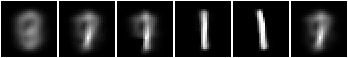
Here are the slices and their underlying for each non-null derived variable state,
let ll = [(w,u) | (ss,_) <- (aall $ hhaa $ hrhh uu2 $ hrc `hrhrred` fder ff), (w,u) <- ssll ss, u /= ValStr("null")]

rpln [hhaa (hrhh uu2 (hrb' `hrhrsel` aahr uu2 rr `hrhrred` (vars rr))) | let hrb' = hrb `hrhrred` (vvk `union` llqq (map fst ll)),  (w,u) <- ll, let rr = single (llss [(w,u)]) 1]
"{({(<<<1,1>,n2>,1>,1)},3643 % 1)}"
"{({(<<<3,1>,n2>,1>,0)},1623 % 1)}"
"{({(<<<8,1>,n2>,1>,1)},775 % 1)}"
"{({(<<<18,1>,n2>,1>,0)},346 % 1)}"
"{({(<<<43,1>,n2>,1>,0)},167 % 1)}"
"{({(<<<105,1>,n2>,1>,0)},121 % 1)}"

bmwrite file $ bmhstack $ map (bmborder 1 . hrbm 28 2 2) $ [hrb' `hrhrsel` aahr uu2 rr `hrhrred` vvk | let hrb' = hrb `hrhrred` (vvk `union` llqq (map fst ll)),  (w,u) <- ll, let rr = single (llss [(w,u)]) 1]

bmwrite file $ bmhstack $ map (bmborder 1 . hrbm 28 2 2) $ [qqhr 2 uu vvk (fund (ff `fdep` sgl w)) | (w,u) <- ll, let rr = single (llss [(w,u)]) 1]

Two level over 15x15 regions
Let us consider a two level model which consists of 5x5 frames of square regions of 15x15 pixels - see Model induction. The model NIST_model25.json is induced by NIST_engine25.hs.
We shall analyse it with the 7,500 events subset of the sample,
:l NISTDev

(uu,hrtr) <- nistTrainBucketedIO 2

let digit = VarStr "digit"
let vv = uvars uu
let vvl = sgl digit
let vvk = vv `minus` vvl

let hr = hrev [i | i <- [0.. hrsize hrtr - 1], i `mod` 8 == 0] hrtr

hrsize hr
7500

df <- dfIO "./NIST_model25.json"

let uu1 = uu `uunion` (fsys (dfff df))

card $ dfund df
602

card $ fder $ dfff df
1341

card $ fvars $ dfff df
5194

let (wmax,lmax,xmax,omax,bmax,mmax,umax,pmax,fmax,mult,seed) = (2^11, 8, 2^10, 30, (30*3), 3, 2^8, 1, 127, 1, 5)

summation mult seed uu1 df hr
(197744.68587714966,96419.64498067372)
The 2-level model is considerably more aligned than the all pixels 1-level model, (129988.66344571306,63698.56389878791).
It has a similar alignment to the 2-level model over 10x10 regions (197806.77675500445,94133.42748410173).
Below is an image of the fud decomposition, and adjacent is an image of the fud underlying superimposed on the slices,
A magnified image of the fud underlying superimposed on the averaged slice, can be seen at Model 25.
We can see that the fud underlying clusters are larger in general than for the 1-level model. The paths vary in length from four fuds to eleven fuds. The tree is more uniform than for the 1-level model. That is, there are fewer effective off-diagonal states.
Let us reduce the 2-level model, $D$, to make it more managable, $D_{\mathrm{r}}$,
let dfr = dfred uu1 df hr

card $ dfund dfr
540

card $ fder $ dfff dfr
127

card $ fvars $ dfff dfr
2401
Let us examine the slices, $P = \mathrm{paths}(A * D_{\mathrm{r}})$,
let pp = qqll $ treesPaths $ hrmult uu1 dfr hr

let variablesVariableFud (VarPair (VarPair (VarPair (f,_),_),_)) = f
    variablesVariableFud _ = VarInt 0

let fid = variablesVariableFud . least . fder

rpln $ zip [0..] $ map (map (fid . snd . fst)) pp
"(0,[1,2,61,118])"
"(1,[1,2,3,14,23,63])"
"(2,[1,2,3,14,23,45,66,95])"
"..."
"(42,[1,5,10,29,53,124])"
"..."
"(47,[1,5,9,15,22,42,72,94])"
"(48,[1,5,9,30,44,62])"
"(49,[1,5,9,30,81,112])"

rpln $ zip [0..] $ map (map (hrsize . snd)) pp
"(0,[7500,5014,3791,2563])"
"(1,[7500,5014,3791,873,446,249])"
"(2,[7500,5014,3791,873,446,197,152,101])"
"..."
"(42,[7500,2486,1329,532,310,125])"
"..."
"(47,[7500,2486,1157,796,501,300,142,114])"
"(48,[7500,2486,1157,361,217,150])"
"(49,[7500,2486,1157,361,144,100])"
Imaging the reduced decomposition slices,
bmwrite file $ bmvstack $ map (\bm -> bminsert (bmempty (28+2) ((28+2)*(maximum (map length pp)))) 0 0 bm) $ map (bmhstack . map (\(_,hrs) -> bmborder 1 (hrbm 28 1 2 (hrs `hrhrred` vvk)))) pp

bmwrite file $ bmvstack $ map (\bm -> bminsert (bmempty (28+2) ((28+2)*(maximum (map length pp)))) 0 0 bm) $ map (bmhstack . map (\((_,ff),hrs) -> bmborder 1 (bmmax (hrbm 28 1 2 (hrs `hrhrred` vvk)) 0 0 (hrbm 28 1 2 (qqhr 2 uu vvk (fund ff)))))) pp
Again, the reduced decomposition is similar to the original decomposition.
The underlying tuple of the root slice is $\mathrm{und}(F)$, where $((\cdot,F),\cdot) = P_{1,1}$,
let ((_,ff),hrs) = pp !! 0 !! 0

card $ fund ff
43

bmwrite file $ bmborder 1 $ bmmax (hrbm 28 3 2 (hrs `hrhrred` vvk)) 0 0 $ hrbm 28 3 2 $ qqhr 2 uu vvk $ fund ff

We can see that the root slice depends on an underlying cluster that is larger than the corresponding cluster for the root slice in the 1-level model. It is also in a different location.
The first child slice of the second column has size 5014,
let ((_,ff),hrs) = pp !! 0 !! 1

card $ fund ff
32

bmwrite file $ bmborder 1 $ bmmax (hrbm 28 3 2 (hrs `hrhrred` vvk)) 0 0 $ hrbm 28 3 2 $ qqhr 2 uu vvk $ fund ff

Again, we can see that the root slice depends on a larger cluster of the substrate than in the 1-level model.
Now let us query the model with a sample event to see how it is being classified. First, consider the fud decomposition fud, $F = D_{\mathrm{r}}^{\mathrm{F}}$,
let ff = dfnul uu1 dfr 2

card $ fvars $ ff
2778

card $ fder $ ff
127

rp $ take 5 $ qqll $ fder $ ff
"[<<<1,1>,n2>,1>,<<<2,1>,n2>,1>,<<<3,1>,n2>,1>,<<<4,1>,n2>,1>,<<<5,1>,n2>,1>]"
Now apply the model to the sample history, $A_{\mathrm{b}} = A * \prod \mathrm{his}(F)$,
let uu2 = uu `uunion` (fsys ff)

let hrb = hrfmul uu2 ff hr

hrsize hrb
7500

card $ hrvars $ hrb
3023
Choose, for example, the first event $Q = \{S\}^{\mathrm{U}}$, where $S \in (A\%V_{\mathrm{k}})^{\mathrm{S}}$,
let hrq = hrev [0] $ hr `hrhrred` vvk

bmwrite file $ bmborder 1 $ hrbm 28 2 2 $ hrq
Now find the leaf slice of the query, $A_{\mathrm{c}} = A_{\mathrm{b}} * (Q * F^{\mathrm{T}})$,
let hrc = hrhrsel hrb $ hrfmul uu2 ff hrq `hrhrred` fder ff

hrsize hrc
150

bmwrite file $ bmborder 1 $ hrbm 28 2 2 $ hrc `hrhrred` vvk

Here are the first 30 slice events, $A_{\mathrm{c}}~\%~V_{\mathrm{k}}$,
bmwrite file $ bmhstack $ map (bmborder 1 . hrbm 28 1 2) $ [hrev [i] hr' | let hr' = hrc `hrhrred` vvk, i <- [0..30-1]]

The label variable is, $A_{\mathrm{c}}~\%~V_{\mathrm{l}}$,
rpln $ aall $ hhaa $ hrhh uu1 $ hrc `hrhrred` vvl
"({(digit,1)},15 % 1)"
"({(digit,2)},17 % 1)"
"({(digit,3)},23 % 1)"
"({(digit,4)},5 % 1)"
"({(digit,5)},13 % 1)"
"({(digit,6)},48 % 1)"
"({(digit,7)},1 % 1)"
"({(digit,8)},27 % 1)"
"({(digit,9)},1 % 1)"
The modal label is six, not five.
Now let us see how the event was chosen. Here are the slices and their underlying for each non-null derived variable state, \[ \{A_{\mathrm{b}} * \{\{(w,u)\}\}^{\mathrm{U}}~\%~\{w\} : (S,\cdot) \in Q * F^{\mathrm{T}},~(w,u) \in S,~u \neq \mathrm{null}\} \]
let hrqb = hrfmul uu2 ff hrq

let ll = [(w,u) | (ss,_) <- (aall $ hhaa $ hrhh uu2 $ hrqb `hrhrred` fder ff), (w,u) <- ssll ss, u /= ValStr("null")]

rpln [hhaa (hrhh uu2 (hrb' `hrhrsel` aahr uu2 rr `hrhrred` (vars rr))) | let hrb' = hrb `hrhrred` (vvk `union` llqq (map fst ll)),  (w,u) <- ll, let rr = single (llss [(w,u)]) 1]
"{({(<<<1,1>,n2>,1>,0)},5014 % 1)}"
"{({(<<<2,1>,n2>,1>,0)},3791 % 1)}"
"{({(<<<3,1>,n2>,1>,0)},873 % 1)}"
"{({(<<<14,1>,n2>,1>,0)},446 % 1)}"
"{({(<<<23,1>,n2>,1>,0)},249 % 1)}"
"{({(<<<61,1>,n2>,1>,0)},1228 % 1)}"
"{({(<<<63,1>,n2>,1>,1)},218 % 1)}"

bmwrite file $ bmhstack $ map (bmborder 1 . hrbm 28 2 2) $ [hrb' `hrhrsel` aahr uu2 rr `hrhrred` vvk | let hrb' = hrb `hrhrred` (vvk `union` llqq (map fst ll)),  (w,u) <- ll, let rr = single (llss [(w,u)]) 1]

bmwrite file $ bmhstack $ map (bmborder 1 . hrbm 28 2 2) $ [qqhr 2 uu vvk (fund (ff `fdep` sgl w)) | (w,u) <- ll, let rr = single (llss [(w,u)]) 1]

Note that we are considering the reduced decomposition, $D_{\mathrm{r}}$, which can be indistinct, so the non-null derived variables do not necessarily correspond to just one path of the original decomposition, $D$. In this case they correspond to two paths,
"(0,[1,2,61,118])"
"(1,[1,2,3,14,23,63])"
"..."

bmwrite file $ bmhstack $ map (\(_,hrs) -> bmborder 1 (hrbm 28 1 2 (hrs `hrhrred` vvk))) $ pp !! 0

bmwrite file $ bmhstack $ map (\(_,hrs) -> bmborder 1 (hrbm 28 1 2 (hrs `hrhrred` vvk))) $ pp !! 1
Let us examine the level 1 nullable derived variables of the central region at (7;7),
let islevnull (VarPair (VarPair (VarPair (_, VarStr "n"), _), VarStr "(7;7)")) = True
    islevnull _ = False

card $ Set.filter islevnull $ fvars $ ff
11

let ll = qqll $ llqq [(w,u) | (ss,_) <- (aall $ hhaa $ hrhh uu2 $ hrqb `hrhrred` Set.filter islevnull (fvars ff)), (w,u) <- ssll ss, u /= ValStr("null")]

rpln [hhaa (hrhh uu2 (hrb' `hrhrsel` aahr uu2 rr `hrhrred` (vars rr))) | let hrb' = hrb `hrhrred` (vvk `union` llqq (map fst ll)),  (w,u) <- ll, let rr = single (llss [(w,u)]) 1]
"{({(<<<<<1,1>,0>,n>,1>,(7;7)>,1)},6525 % 1)}"
"{({(<<<<<1,2>,0>,n>,1>,(7;7)>,0)},1600 % 1)}"

bmwrite file $ bmhstack $ map (bmborder 1 . hrbm 28 2 2) $ [hrb' `hrhrsel` aahr uu2 rr `hrhrred` vvk | let hrb' = hrb `hrhrred` (vvk `union` llqq (map fst ll)),  (w,u) <- ll, let rr = single (llss [(w,u)]) 1]

let bmmask = bminsert (bmempty (28*2) (28*2)) (((28-15-7)*2)-1) ((7*2)-1) (bmfull (15*2) (15*2))

bmwrite file $ bmhstack $ map (bmborder 1 . bmmin bmmask 0 0 . hrbm 28 2 2) $ [hrb' `hrhrsel` aahr uu2 rr `hrhrred` vvk | let hrb' = hrb `hrhrred` (vvk `union` llqq (map fst ll)),  (w,u) <- ll, let rr = single (llss [(w,u)]) 1]

bmwrite file $ bmhstack $ map (bmborder 1 . hrbm 28 2 2) $ [qqhr 2 uu vvk (fund (ff `fdep` sgl w)) | (w,u) <- ll, let rr = single (llss [(w,u)]) 1]

This frame detects the middle section of the five.
We can compare this region to the region, say, at (1;13),
let islevnull (VarPair (VarPair (VarPair (_, VarStr "n"), _), VarStr "(1;13)")) = True
    islevnull _ = False

card $ Set.filter islevnull $ fvars $ ff
9

let ll = qqll $ llqq [(w,u) | (ss,_) <- (aall $ hhaa $ hrhh uu2 $ hrqb `hrhrred` Set.filter islevnull (fvars ff)), (w,u) <- ssll ss, u /= ValStr("null")]

rpln [hhaa (hrhh uu2 (hrb' `hrhrsel` aahr uu2 rr `hrhrred` (vars rr))) | let hrb' = hrb `hrhrred` (vvk `union` llqq (map fst ll)),  (w,u) <- ll, let rr = single (llss [(w,u)]) 1]
"{({(<<<<<1,1>,0>,n>,1>,(1;13)>,0)},6011 % 1)}"
"{({(<<<<<1,4>,0>,n>,1>,(1;13)>,1)},3991 % 1)}"
"{({(<<<<<1,7>,0>,n>,1>,(1;13)>,1)},202 % 1)}"
"{({(<<<<<1,100>,0>,n>,1>,(1;13)>,0)},5782 % 1)}"

bmwrite file $ bmhstack $ map (bmborder 1 . hrbm 28 2 2) $ [hrb' `hrhrsel` aahr uu2 rr `hrhrred` vvk | let hrb' = hrb `hrhrred` (vvk `union` llqq (map fst ll)),  (w,u) <- ll, let rr = single (llss [(w,u)]) 1]

let bmmask = bminsert (bmempty (28*2) (28*2)) (((28-15-1)*2)-1) ((13*2)-1) (bmfull (15*2) (15*2))

bmwrite file $ bmhstack $ map (bmborder 1 . bmmin bmmask 0 0 . hrbm 28 2 2) $ [hrb' `hrhrsel` aahr uu2 rr `hrhrred` vvk | let hrb' = hrb `hrhrred` (vvk `union` llqq (map fst ll)),  (w,u) <- ll, let rr = single (llss [(w,u)]) 1]

bmwrite file $ bmhstack $ map (bmborder 1 . hrbm 28 2 2) $ [qqhr 2 uu vvk (fund (ff `fdep` sgl w)) | (w,u) <- ll, let rr = single (llss [(w,u)]) 1]

This frame detects the top right tip of the five.
We can compare again to the region at (4;7),
let islevnull (VarPair (VarPair (VarPair (_, VarStr "n"), _), VarStr "(4;7)")) = True
    islevnull _ = False

card $ Set.filter islevnull $ fvars $ ff
11

let ll = qqll $ llqq [(w,u) | (ss,_) <- (aall $ hhaa $ hrhh uu2 $ hrqb `hrhrred` Set.filter islevnull (fvars ff)), (w,u) <- ssll ss, u /= ValStr("null")]

rpln [hhaa (hrhh uu2 (hrb' `hrhrsel` aahr uu2 rr `hrhrred` (vars rr))) | let hrb' = hrb `hrhrred` (vvk `union` llqq (map fst ll)),  (w,u) <- ll, let rr = single (llss [(w,u)]) 1]
"{({(<<<<<1,1>,0>,n>,1>,(4;7)>,0)},1300 % 1)}"
"{({(<<<<<1,4>,0>,n>,1>,(4;7)>,1)},786 % 1)}"
"{({(<<<<<1,100>,0>,n>,1>,(4;7)>,1)},909 % 1)}"

bmwrite file $ bmhstack $ map (bmborder 1 . hrbm 28 2 2) $ [hrb' `hrhrsel` aahr uu2 rr `hrhrred` vvk | let hrb' = hrb `hrhrred` (vvk `union` llqq (map fst ll)),  (w,u) <- ll, let rr = single (llss [(w,u)]) 1]

let bmmask = bminsert (bmempty (28*2) (28*2)) (((28-15-4)*2)-1) ((7*2)-1) (bmfull (15*2) (15*2))

bmwrite file $ bmhstack $ map (bmborder 1 . bmmin bmmask 0 0 . hrbm 28 2 2) $ [hrb' `hrhrsel` aahr uu2 rr `hrhrred` vvk | let hrb' = hrb `hrhrred` (vvk `union` llqq (map fst ll)),  (w,u) <- ll, let rr = single (llss [(w,u)]) 1]

bmwrite file $ bmhstack $ map (bmborder 1 . hrbm 28 2 2) $ [qqhr 2 uu vvk (fund (ff `fdep` sgl w)) | (w,u) <- ll, let rr = single (llss [(w,u)]) 1]

This frame detects the top arc of the five.
Now let us repeat the same analysis for the next event,
let hrq = hrev [1] $ hr `hrhrred` vvk

bmwrite file $ bmborder 1 $ hrbm 28 2 2 $ hrq
Now find the leaf slice of the query,
let hrc = hrhrsel hrb $ hrfmul uu2 ff hrq `hrhrred` fder ff

hrsize hrc
80

bmwrite file $ bmborder 1 $ hrbm 28 2 2 $ hrc `hrhrred` vvk

Here are the first 20 slice events,
bmwrite file $ bmhstack $ map (bmborder 1 . hrbm 28 1 2) $ [hrev [i] hr' | let hr' = hrc `hrhrred` vvk, i <- [0..20-1]]

The label variable is,
rpln $ aall $ hhaa $ hrhh uu1 $ hrc `hrhrred` vvl
"({(digit,1)},79 % 1)"
"({(digit,9)},1 % 1)"
In this case the slice consists of nearly all ones.
Here are the slices and their underlying for each non-null derived variable state,
let ll = [(w,u) | (ss,_) <- (aall $ hhaa $ hrhh uu2 $ hrc `hrhrred` fder ff), (w,u) <- ssll ss, u /= ValStr("null")]

rpln [hhaa (hrhh uu2 (hrb' `hrhrsel` aahr uu2 rr `hrhrred` (vars rr))) | let hrb' = hrb `hrhrred` (vvk `union` llqq (map fst ll)),  (w,u) <- ll, let rr = single (llss [(w,u)]) 1]
"{({(<<<1,1>,n2>,1>,1)},2486 % 1)}"
"{({(<<<5,1>,n2>,1>,0)},1329 % 1)}"
"{({(<<<10,1>,n2>,1>,1)},532 % 1)}"
"{({(<<<29,1>,n2>,1>,1)},310 % 1)}"
"{({(<<<53,1>,n2>,1>,0)},125 % 1)}"
"{({(<<<124,1>,n2>,1>,0)},80 % 1)}"

bmwrite file $ bmhstack $ map (bmborder 1 . hrbm 28 2 2) $ [hrb' `hrhrsel` aahr uu2 rr `hrhrred` vvk | let hrb' = hrb `hrhrred` (vvk `union` llqq (map fst ll)),  (w,u) <- ll, let rr = single (llss [(w,u)]) 1]

bmwrite file $ bmhstack $ map (bmborder 1 . hrbm 28 2 2) $ [qqhr 2 uu vvk (fund (ff `fdep` sgl w)) | (w,u) <- ll, let rr = single (llss [(w,u)]) 1]

Two level over centred square regions of 11x11 pixels
Let us consider a two level model which consists of 5x5 frames of Centred square regions of 11x11 pixels - see Model induction. The model NIST_model26.json is induced by NIST_engine26.hs.
We shall analyse it with the 7,500 events subset of the sample,
:l NISTDev

(uu,hrtr) <- nistTrainBucketedIO 2

let digit = VarStr "digit"
let vv = uvars uu
let vvl = sgl digit
let vvk = vv `minus` vvl

let hr = hrev [i | i <- [0.. hrsize hrtr - 1], i `mod` 8 == 0] hrtr

hrsize hr
7500

df <- dfIO "./NIST_model26.json"

let uu1 = uu `uunion` (fsys (dfff df))

card $ dfund df
586

card $ fder $ dfff df
1348

card $ fvars $ dfff df
7701

let (wmax,lmax,xmax,omax,bmax,mmax,umax,pmax,fmax,mult,seed) = (2^11, 8, 2^10, 30, (30*3), 3, 2^8, 1, 127, 1, 5)

summation mult seed uu1 df hr
(158648.91674670018,78295.49235393995)
We can compare this to the all pixels 1-level model, (129988.66344571306,63698.56389878791). The 2-level model is more highly aligned, but the difference is less than the non-centred 2-level models, Two level over 10x10 regions, (197806.77675500445,94133.42748410173), and Two level over 15x15 regions, (197744.68587714966,96419.64498067372).
Below is an image of the fud decomposition, and adjacent is an image of the fud underlying superimposed on the slices,
A magnified image of the fud underlying superimposed on the averaged slice, can be seen at Model 26.
We can see that the fud underlying clusters are larger in general than for the 1-level model. The paths vary in length from three fuds to 24 fuds. The tree is a little more uniform than the 1-level model, reflected in the higher alignment. The tree is less uniform than for the other 2-level models, Two level over 10x10 regions and Two level over 15x15 regions.
Let us reduce the 2-level model, $D$, to make it more managable, $D_{\mathrm{r}}$,
let dfr = dfred uu1 df hr

card $ dfund dfr
541

card $ fder $ dfff dfr
127

card $ fvars $ dfff dfr
3960
Let us examine the slices, $P = \mathrm{paths}(A * D_{\mathrm{r}})$,
let pp = qqll $ treesPaths $ hrmult uu1 dfr hr

let variablesVariableFud (VarPair (VarPair (VarPair (f,_),_),_)) = f
    variablesVariableFud _ = VarInt 0

let fid = variablesVariableFud . least . fder

rpln $ zip [0..] $ map (map (fid . snd . fst)) pp
"(0,[1,2,3,4,5,7,8,10,12,16,20,23,25,29,32,35,40,54,58,76,89,106,113,125])"
"(1,[1,2,3,4,5,7,8,10,12,16,20,23,25,91,102])"
"(2,[1,2,3,4,5,7,8,10,12,16,20,120])"
"..."
"(14,[1,2,3,78,87,111])"
"..."
"(23,[1,2,101])"
"..."
"(27,[1,2,6,19,51,62])"
"..."
"(42,[1,9,13,14,41,127])"
"(43,[1,9,13,44,88])"
"(44,[1,9,45,69])"

rpln $ zip [0..] $ map (map (hrsize . snd)) pp
"(0,[7500,6215,4508,3060,2708,2348,1968,1529,1378,1144,905,792,727,585,496,425,380,323,287,238,189,172,157,149])"
"(1,[7500,6215,4508,3060,2708,2348,1968,1529,1378,1144,905,792,727,142,124])"
"(2,[7500,6215,4508,3060,2708,2348,1968,1529,1378,1144,905,113])"
"..."
"(14,[7500,6215,4508,3060,2780,2583])"
"..."
"(23,[7500,6215,1707])"
"..."
"(27,[7500,6215,1707,756,263,205])"
"..."
"(42,[7500,1285,1122,956,245,106])"
"(43,[7500,1285,1122,166,66])"
"(44,[7500,1285,163,128])"
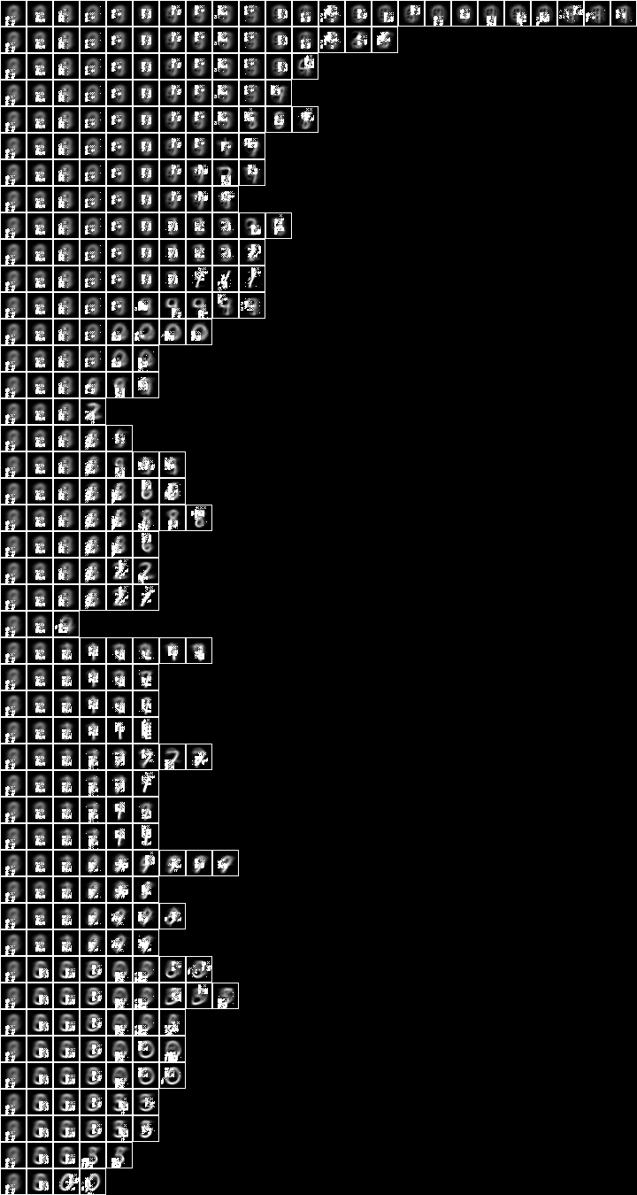
Imaging the reduced decomposition slices,
bmwrite file $ bmvstack $ map (\bm -> bminsert (bmempty (28+2) ((28+2)*(maximum (map length pp)))) 0 0 bm) $ map (bmhstack . map (\(_,hrs) -> bmborder 1 (hrbm 28 1 2 (hrs `hrhrred` vvk)))) pp

bmwrite file $ bmvstack $ map (\bm -> bminsert (bmempty (28+2) ((28+2)*(maximum (map length pp)))) 0 0 bm) $ map (bmhstack . map (\((_,ff),hrs) -> bmborder 1 (bmmax (hrbm 28 1 2 (hrs `hrhrred` vvk)) 0 0 (hrbm 28 1 2 (qqhr 2 uu vvk (fund ff)))))) pp

Again, the reduced decomposition is similar to the original decomposition.
The underlying tuple of the root slice is $\mathrm{und}(F)$, where $((\cdot,F),\cdot) = P_{1,1}$,
let ((_,ff),hrs) = pp !! 0 !! 0

card $ fund ff
44

bmwrite file $ bmborder 1 $ bmmax (hrbm 28 3 2 (hrs `hrhrred` vvk)) 0 0 $ hrbm 28 3 2 $ qqhr 2 uu vvk $ fund ff

We can see that the root slice depends on an underlying cluster that is larger than the corresponding cluster for the root slice in the 1-level model. It is also in a different location.
The first child slice of the second column has size 6215,
let ((_,ff),hrs) = pp !! 0 !! 1

card $ fund ff
59

bmwrite file $ bmborder 1 $ bmmax (hrbm 28 3 2 (hrs `hrhrred` vvk)) 0 0 $ hrbm 28 3 2 $ qqhr 2 uu vvk $ fund ff

Again, we can see that the root slice depends on a larger cluster of the substrate than in the 1-level model.
Now let us query the model with a sample event to see how it is being classified. First, consider the fud decomposition fud, $F = D_{\mathrm{r}}^{\mathrm{F}}$,
let ff = dfnul uu1 dfr 2

card $ fvars $ ff
4337

card $ fder $ ff
127

rp $ take 5 $ qqll $ fder $ ff
"[<<<1,1>,n2>,1>,<<<2,1>,n2>,1>,<<<3,1>,n2>,1>,<<<4,1>,n2>,1>,<<<5,1>,n2>,1>]"
Now apply the model to the sample history, $A_{\mathrm{b}} = A * \prod \mathrm{his}(F)$,
let uu2 = uu `uunion` (fsys ff)

let hrb = hrfmul uu2 ff hr

hrsize hrb
7500

card $ hrvars $ hrb
4581
Choose, for example, the first event $Q = \{S\}^{\mathrm{U}}$, where $S \in (A\%V_{\mathrm{k}})^{\mathrm{S}}$,
let hrq = hrev [0] $ hr `hrhrred` vvk

bmwrite file $ bmborder 1 $ hrbm 28 2 2 $ hrq
Now find the leaf slice of the query, $A_{\mathrm{c}} = A_{\mathrm{b}} * (Q * F^{\mathrm{T}})$,
let hrc = hrhrsel hrb $ hrfmul uu2 ff hrq `hrhrred` fder ff

hrsize hrc
67

bmwrite file $ bmborder 1 $ hrbm 28 2 2 $ hrc `hrhrred` vvk

Here are the first 30 slice events, $A_{\mathrm{c}}~\%~V_{\mathrm{k}}$,
bmwrite file $ bmhstack $ map (bmborder 1 . hrbm 28 1 2) $ [hrev [i] hr' | let hr' = hrc `hrhrred` vvk, i <- [0..30-1]]

The label variable is, $A_{\mathrm{c}}~\%~V_{\mathrm{l}}$,
rpln $ aall $ hhaa $ hrhh uu1 $ hrc `hrhrred` vvl
"({(digit,2)},1 % 1)"
"({(digit,3)},22 % 1)"
"({(digit,4)},3 % 1)"
"({(digit,5)},11 % 1)"
"({(digit,6)},13 % 1)"
"({(digit,7)},1 % 1)"
"({(digit,8)},9 % 1)"
"({(digit,9)},7 % 1)"
The modal label is three, not five.
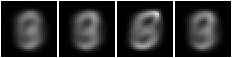
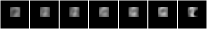
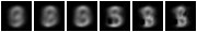
Now let us see how the event was chosen. Here are the slices and their underlying for each non-null derived variable state, \[ \{A_{\mathrm{b}} * \{\{(w,u)\}\}^{\mathrm{U}}~\%~\{w\} : (S,\cdot) \in Q * F^{\mathrm{T}},~(w,u) \in S,~u \neq \mathrm{null}\} \]
let hrqb = hrfmul uu2 ff hrq

let ll = [(w,u) | (ss,_) <- (aall $ hhaa $ hrhh uu2 $ hrqb `hrhrred` fder ff), (w,u) <- ssll ss, u /= ValStr("null")]

rpln [hhaa (hrhh uu2 (hrb' `hrhrsel` aahr uu2 rr `hrhrred` (vars rr))) | let hrb' = hrb `hrhrred` (vvk `union` llqq (map fst ll)),  (w,u) <- ll, let rr = single (llss [(w,u)]) 1]
"{({(<<<1,1>,n2>,1>,0)},6215 % 1)}"
"{({(<<<2,1>,n2>,1>,0)},4508 % 1)}"
"{({(<<<3,1>,n2>,1>,0)},3060 % 1)}"
"{({(<<<4,1>,n2>,1>,0)},2708 % 1)}"
"{({(<<<5,1>,n2>,1>,0)},2348 % 1)}"
"{({(<<<7,1>,n2>,1>,0)},1968 % 1)}"
"{({(<<<8,1>,n2>,1>,0)},1529 % 1)}"
"{({(<<<10,1>,n2>,1>,0)},1378 % 1)}"
"{({(<<<12,1>,n2>,1>,0)},1144 % 1)}"
"{({(<<<16,1>,n2>,1>,0)},905 % 1)}"
"{({(<<<20,1>,n2>,1>,0)},792 % 1)}"
"{({(<<<23,1>,n2>,1>,0)},727 % 1)}"
"{({(<<<25,1>,n2>,1>,0)},585 % 1)}"
"{({(<<<29,1>,n2>,1>,0)},496 % 1)}"
"{({(<<<32,1>,n2>,1>,1)},71 % 1)}"
"{({(<<<78,1>,n2>,1>,0)},2780 % 1)}"
"{({(<<<87,1>,n2>,1>,0)},2583 % 1)}"
"{({(<<<111,1>,n2>,1>,0)},2511 % 1)}"

bmwrite file $ bmhstack $ map (bmborder 1 . hrbm 28 2 2) $ [hrb' `hrhrsel` aahr uu2 rr `hrhrred` vvk | let hrb' = hrb `hrhrred` (vvk `union` llqq (map fst ll)),  (w,u) <- ll, let rr = single (llss [(w,u)]) 1]

bmwrite file $ bmhstack $ map (bmborder 1 . hrbm 28 2 2) $ [qqhr 2 uu vvk (fund (ff `fdep` sgl w)) | (w,u) <- ll, let rr = single (llss [(w,u)]) 1]


Note that we are considering the reduced decomposition, $D_{\mathrm{r}}$, which can be indistinct, so the non-null derived variables do not necessarily correspond to just one path of the original decomposition, $D$. In this case they correspond to two paths,
"(0,[1,2,3,4,5,7,8,10,12,16,20,23,25,29,32,35,40,54,58,76,89,106,113,125])"
"..."
"(14,[1,2,3,78,87,111])"

bmwrite file $ bmhstack $ map (\(_,hrs) -> bmborder 1 (hrbm 28 1 2 (hrs `hrhrred` vvk))) $ pp !! 0

bmwrite file $ bmhstack $ map (\(_,hrs) -> bmborder 1 (hrbm 28 1 2 (hrs `hrhrred` vvk))) $ pp !! 14

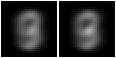
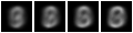
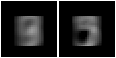
Let us examine the level 1 nullable derived variables of the central region at (10;10),
let islevnull (VarPair (VarPair (VarPair (_, VarStr "n"), _), VarStr "(10;10)")) = True
    islevnull _ = False

card $ Set.filter islevnull $ fvars $ ff
39

let ll = qqll $ llqq [(w,u) | (ss,_) <- (aall $ hhaa $ hrhh uu2 $ hrqb `hrhrred` Set.filter islevnull (fvars ff)), (w,u) <- ssll ss, u /= ValStr("null")]

rpln [hhaa (hrhh uu2 (hrb' `hrhrsel` aahr uu2 rr `hrhrred` (vars rr))) | let hrb' = hrb `hrhrred` (vvk `union` llqq (map fst ll)),  (w,u) <- ll, let rr = single (llss [(w,u)]) 1]
"{({(<<<<<1,0>,0>,n>,1>,(10;10)>,1)},3763 % 1)}"
"{({(<<<<<1,1>,0>,n>,1>,(10;10)>,1)},2896 % 1)}"
"{({(<<<<<1,7>,0>,n>,1>,(10;10)>,1)},553 % 1)}"
"{({(<<<<<1,9>,0>,n>,1>,(10;10)>,1)},205 % 1)}"
"{({(<<<<<1,26>,0>,n>,1>,(10;10)>,0)},1178 % 1)}"
"{({(<<<<<1,60>,0>,n>,1>,(10;10)>,1)},510 % 1)}"
"{({(<<<<<1,63>,0>,n>,1>,(10;10)>,1)},1538 % 1)}"
"{({(<<<<<1,77>,0>,n>,1>,(10;10)>,1)},1657 % 1)}"
"{({(<<<<<1,89>,0>,n>,1>,(10;10)>,1)},1444 % 1)}"
"{({(<<<<<1,109>,0>,n>,1>,(10;10)>,1)},1931 % 1)}"

bmwrite file $ bmhstack $ map (bmborder 1 . hrbm 28 2 2) $ [hrb' `hrhrsel` aahr uu2 rr `hrhrred` vvk | let hrb' = hrb `hrhrred` (vvk `union` llqq (map fst ll)),  (w,u) <- ll, let rr = single (llss [(w,u)]) 1]

let bmmask = bminsert (bmempty (28*2) (28*2)) (((28-11-10)*2)-1) ((10*2)-1) (bmfull (11*2) (11*2))

bmwrite file $ bmhstack $ map (bmborder 1 . bmmin bmmask 0 0 . hrbm 28 2 2) $ [hrb' `hrhrsel` aahr uu2 rr `hrhrred` vvk | let hrb' = hrb `hrhrred` (vvk `union` llqq (map fst ll)),  (w,u) <- ll, let rr = single (llss [(w,u)]) 1]

bmwrite file $ bmhstack $ map (bmborder 1 . hrbm 28 2 2) $ [qqhr 2 uu vvk (fund (ff `fdep` sgl w)) | (w,u) <- ll, let rr = single (llss [(w,u)]) 1]

This frame detects the middle section of the five.
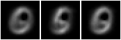
We can compare this region to the region, say, at (2;18),
let islevnull (VarPair (VarPair (VarPair (_, VarStr "n"), _), VarStr "(2;18)")) = True
    islevnull _ = False

card $ Set.filter islevnull $ fvars $ ff
1

let ll = qqll $ llqq [(w,u) | (ss,_) <- (aall $ hhaa $ hrhh uu2 $ hrqb `hrhrred` Set.filter islevnull (fvars ff)), (w,u) <- ssll ss, u /= ValStr("null")]

rpln [hhaa (hrhh uu2 (hrb' `hrhrsel` aahr uu2 rr `hrhrred` (vars rr))) | let hrb' = hrb `hrhrred` (vvk `union` llqq (map fst ll)),  (w,u) <- ll, let rr = single (llss [(w,u)]) 1]
"{({(<<<<<1,0>,0>,n>,1>,(2;18)>,1)},325 % 1)}"

bmwrite file $ bmhstack $ map (bmborder 1 . hrbm 28 2 2) $ [hrb' `hrhrsel` aahr uu2 rr `hrhrred` vvk | let hrb' = hrb `hrhrred` (vvk `union` llqq (map fst ll)),  (w,u) <- ll, let rr = single (llss [(w,u)]) 1]

let bmmask = bminsert (bmempty (28*2) (28*2)) (((28-11-2)*2)-1) ((18*2)-1) (bmfull (11*2) (11*2))

bmwrite file $ bmhstack $ map (bmborder 1 . bmmin bmmask 0 0 . hrbm 28 2 2) $ [hrb' `hrhrsel` aahr uu2 rr `hrhrred` vvk | let hrb' = hrb `hrhrred` (vvk `union` llqq (map fst ll)),  (w,u) <- ll, let rr = single (llss [(w,u)]) 1]

bmwrite file $ bmhstack $ map (bmborder 1 . hrbm 28 2 2) $ [qqhr 2 uu vvk (fund (ff `fdep` sgl w)) | (w,u) <- ll, let rr = single (llss [(w,u)]) 1]


This frame detects the top right tip of the five. In this case the central pixel is set, but no other non-null level-1 derived variables happen to be included.
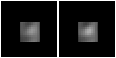
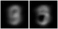
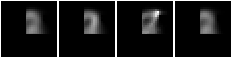
We can compare again to the region at (6;10),
let islevnull (VarPair (VarPair (VarPair (_, VarStr "n"), _), VarStr "(6;10)")) = True
    islevnull _ = False

card $ Set.filter islevnull $ fvars $ ff
24

let ll = qqll $ llqq [(w,u) | (ss,_) <- (aall $ hhaa $ hrhh uu2 $ hrqb `hrhrred` Set.filter islevnull (fvars ff)), (w,u) <- ssll ss, u /= ValStr("null")]

rpln [hhaa (hrhh uu2 (hrb' `hrhrsel` aahr uu2 rr `hrhrred` (vars rr))) | let hrb' = hrb `hrhrred` (vvk `union` llqq (map fst ll)),  (w,u) <- ll, let rr = single (llss [(w,u)]) 1]
"{({(<<<<<1,0>,0>,n>,1>,(6;10)>,0)},5268 % 1)}"

bmwrite file $ bmhstack $ map (bmborder 1 . hrbm 28 2 2) $ [hrb' `hrhrsel` aahr uu2 rr `hrhrred` vvk | let hrb' = hrb `hrhrred` (vvk `union` llqq (map fst ll)),  (w,u) <- ll, let rr = single (llss [(w,u)]) 1]

let bmmask = bminsert (bmempty (28*2) (28*2)) (((28-11-6)*2)-1) ((10*2)-1) (bmfull (11*2) (11*2))

bmwrite file $ bmhstack $ map (bmborder 1 . bmmin bmmask 0 0 . hrbm 28 2 2) $ [hrb' `hrhrsel` aahr uu2 rr `hrhrred` vvk | let hrb' = hrb `hrhrred` (vvk `union` llqq (map fst ll)),  (w,u) <- ll, let rr = single (llss [(w,u)]) 1]

bmwrite file $ bmhstack $ map (bmborder 1 . hrbm 28 2 2) $ [qqhr 2 uu vvk (fund (ff `fdep` sgl w)) | (w,u) <- ll, let rr = single (llss [(w,u)]) 1]


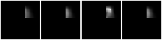
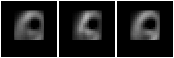
This frame detects the top arc of the five. In this case the central pixel is not set, so the underlying consists solely of that pixel in this centred model.
Now let us repeat the same analysis for the next event,
let hrq = hrev [1] $ hr `hrhrred` vvk

bmwrite file $ bmborder 1 $ hrbm 28 2 2 $ hrq
Now find the leaf slice of the query,
let hrc = hrhrsel hrb $ hrfmul uu2 ff hrq `hrhrred` fder ff

hrsize hrc
58

bmwrite file $ bmborder 1 $ hrbm 28 2 2 $ hrc `hrhrred` vvk

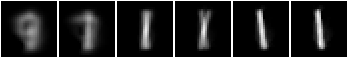
Here are the first 20 slice events,
bmwrite file $ bmhstack $ map (bmborder 1 . hrbm 28 1 2) $ [hrev [i] hr' | let hr' = hrc `hrhrred` vvk, i <- [0..20-1]]

The label variable is,
rpln $ aall $ hhaa $ hrhh uu1 $ hrc `hrhrred` vvl
"({(digit,1)},58 % 1)"
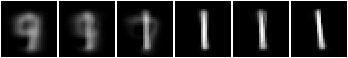
In this case the entire slice consists of ones.
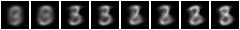
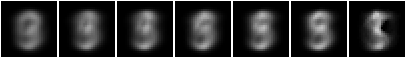
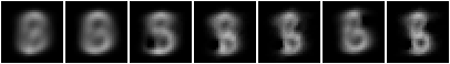
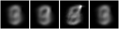
Here are the slices and their underlying for each non-null derived variable state,
let ll = [(w,u) | (ss,_) <- (aall $ hhaa $ hrhh uu2 $ hrc `hrhrred` fder ff), (w,u) <- ssll ss, u /= ValStr("null")]

rpln [hhaa (hrhh uu2 (hrb' `hrhrsel` aahr uu2 rr `hrhrred` (vars rr))) | let hrb' = hrb `hrhrred` (vvk `union` llqq (map fst ll)),  (w,u) <- ll, let rr = single (llss [(w,u)]) 1]
"{({(<<<1,1>,n2>,1>,0)},6215 % 1)}"
"{({(<<<2,1>,n2>,1>,1)},1707 % 1)}"
"{({(<<<6,1>,n2>,1>,0)},756 % 1)}"
"{({(<<<19,1>,n2>,1>,1)},263 % 1)}"
"{({(<<<51,1>,n2>,1>,1)},58 % 1)}"
"{({(<<<101,1>,n2>,1>,0)},1591 % 1)}"

bmwrite file $ bmhstack $ map (bmborder 1 . hrbm 28 2 2) $ [hrb' `hrhrsel` aahr uu2 rr `hrhrred` vvk | let hrb' = hrb `hrhrred` (vvk `union` llqq (map fst ll)),  (w,u) <- ll, let rr = single (llss [(w,u)]) 1]

bmwrite file $ bmhstack $ map (bmborder 1 . hrbm 28 2 2) $ [qqhr 2 uu vvk (fund (ff `fdep` sgl w)) | (w,u) <- ll, let rr = single (llss [(w,u)]) 1]