Induced models
MNIST - handwritten digits/Induced models
Sections
Square regions of 10x10 pixels
Square regions of 15x15 pixels
Centred square regions of 11x11 pixels
Two level over centred square regions of 11x11 pixels
Introduction
Consider an unsupervised induced model $D$ on the query variables, $V_{\mathrm{k}}$, which exclude digit. Later we shall analyse this model, $D$, to find a smaller semi-supervised submodel that predicts the label variables, $V_{\mathrm{l}}$, or digit. In this section, however, we will aim to optimise unsupervised model likelihood by maximising alignment.
Here the induced model is created by the limited-nodes highest-layer excluded-self maximum-roll-by-derived-dimension fud decomper, $(\cdot,D) = I_{P,U,\mathrm{D,F,mm,xs,d,f}}((V_{\mathrm{k}},A))$.
There are some examples of model induction in the NIST repository.
15-fud model
Consider a 15-fud induced model NIST_model2.json of 7,500 events of the training sample, see Model 2. First, load the sample,
from NISTDev import *

(uu,hrtr) = nistTrainBucketedIO(2)

digit = VarStr("digit")
vv = uvars(uu)
vvl = sset([digit])
vvk = vv - vvl

hr = hrev([i for i in range(hrsize(hrtr)) if i % 8 == 0],hrtr)
Now load the model using the utility dfIO in module NISTDev,
df = dfIO('./NIST_model2.json')

uu1 = uunion(uu,fsys(dfff(df)))

len(dfund(df))
134

len(fvars(dfff(df)))
515
We can calculate its summed alignment and the summed alignment valency-density, $\mathrm{summation}(U_{1},D,A))$,
(wmax,lmax,xmax,omax,bmax,mmax,umax,pmax,fmax,mult,seed) = (2**10, 8, 2**10, 10, (10*3), 3, 2**8, 1, 15, 3, 5)

summation(mult,seed,uu1,df,hr)
# (137828.7038275605, 68687.36371089712)
Let us analyse the fud decomposition. Let $P = \mathrm{paths}(A * D)$,
pp = treesPaths(hrmult(uu1,df,hr))

rpln([[hrsize(hr) for (_,hr) in ll] for ll in pp])
# [7500, 2584, 1043]
# [7500, 2584, 1540, 602]
# [7500, 4619, 1575, 672]
# [7500, 4619, 2966, 1157, 609]
# [7500, 4619, 2966, 1804, 813]
# [7500, 4619, 2966, 1804, 986, 583]
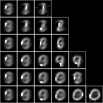
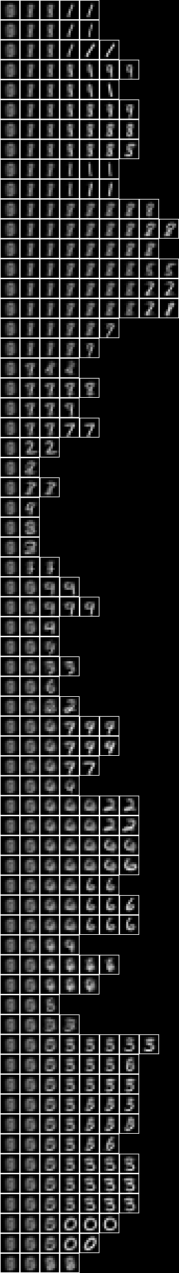
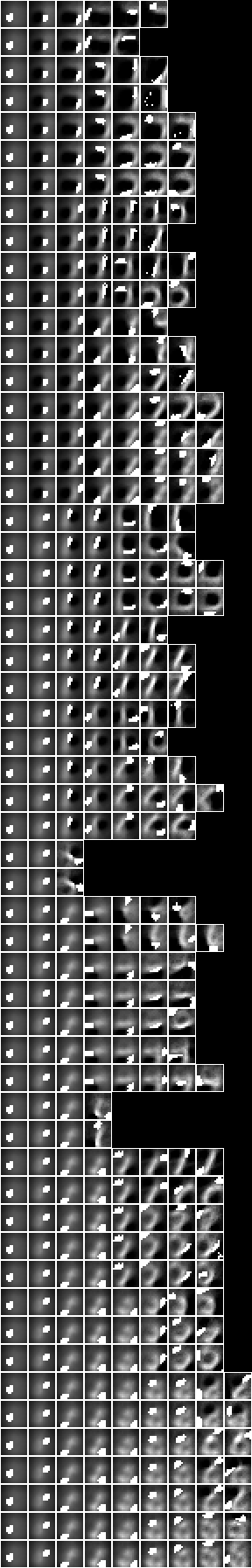
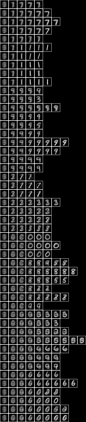
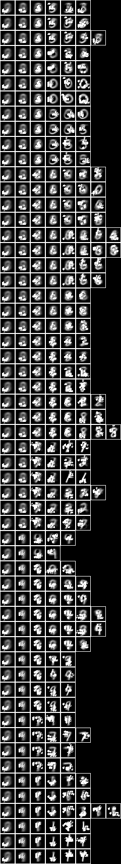
Let us image the fud decomposition,
file = "NIST.bmp"

bmwrite(file,ppbm(uu,vvk,28,2,2,pp))
The bitmap helper function, ppbm, is defined in NISTDev,
def ppbm(uu,vvk,b,c,d,pp):
    kk = []
    for ll in pp:
        jj = []
        for ((_,ff),hrs) in ll:
            jj.append(bmborder(1,bmmax(hrbm(b,c,d,hrhrred(hrs,vvk)),0,0,hrbm(b,c,d,qqhr(d,uu,vvk,fund(ff))))))
        kk.append(bminsert(bmempty((b*c)+2,((b*c)+2)*max([len(ii) for ii in pp])),0,0,bmhstack(jj)))
    return bmvstack(kk)
Here we have shown the fud decomposition, $D$, as a vertical stack of decomposition paths of averaged slice images. Each path runs horizontally from the root slice on the left to the leaf slice on the right. The fud underlying variables are also shown superimposed on each slice image. This shows where the ‘attention’ is during decomposition along a path.
The leftmost column contains only the root slice, which is the entire sample of 7500 events. We can also see the root fud underlying variables shown superimposed on the averaged root slice. The underlying tuple here is $\mathrm{und}(F)$, where $((\cdot,F),\cdot) = P_{1,1}$,
((_,ff),hrs) = pp[0][0]

fund(ff)
# {<10,9>, <10,10>, <10,11>, <11,9>, <11,10>, <11,11>, <12,9>, <12,10>, <12,11>, <13,9>, <13,10>, <14,9>, <14,10>, <15,9>}

bmwrite(file,bmborder(1,bmmax(hrbm(28,3,2,hrhrred(hrs,vvk)),0,0,hrbm(28,3,2,qqhr(2,uu,vvk,fund(ff))))))

It is similar to the first tuple of the investigation of the properties of the sample using the tupler, above.
The second column consists of two children fuds of slice size 2584 and slice size 4619. The first slice is open on the left side of the top loop. It has underlying tuple,
((_,ff),hrs) = pp[0][1]

fund(ff)
# {<10,15>, <10,16>, <11,15>, <11,16>, <12,15>, <12,16>, <13,15>, <13,16>, <14,14>, <14,15>, <14,16>, <15,15>}

bmwrite(file,bmborder(1,bmmax(hrbm(28,3,2,hrhrred(hrs,vvk)),0,0,hrbm(28,3,2,qqhr(2,uu,vvk,fund(ff))))))

The first three rows of the third column consists of two children fuds of slice size 1043 and slice size 1540. The first slice looks more like a one than a two or a three now. It has underlying tuple,
((_,ff),hrs) = pp[0][2]

fund(ff)
# {<10,16>, <10,25>, <11,15>, <11,16>, <12,15>, <12,16>, <13,4>, <13,15>, <13,16>, <14,15>, <14,16>, <15,15>, <26,23>}

bmwrite(file,bmborder(1,bmmax(hrbm(28,3,2,hrhrred(hrs,vvk)),0,0,hrbm(28,3,2,qqhr(2,uu,vvk,fund(ff))))))

Following the first row from left to right, we see where the alignments are maximised at each step of the decomposition.
All pixels
Now consider a 127-fud induced model of the 60,000 events of the training sample NIST_model35.json which is induced by NIST_engine35.py, see Model 35.
We shall analyse it with the 7,500 events subset of the sample,
from NISTDev import *

(uu,hrtr) = nistTrainBucketedIO(2)

digit = VarStr("digit")
vv = uvars(uu)
vvl = sset([digit])
vvk = vv - vvl

hr = hrev([i for i in range(hrsize(hrtr)) if i % 8 == 0],hrtr)

hrsize(hr)
7500

df = dfIO('./NIST_model35.json')

uu1 = uunion(uu,fsys(dfff(df)))

len(dfund(df))
488

len(fvars(dfff(df)))
4040

(wmax,lmax,xmax,omax,bmax,mmax,umax,pmax,fmax,mult,seed) = (2**11, 8, 2**10, 30, (30*3), 3, 2**8, 1, 127, 1, 5)

summation(mult,seed,uu1,df,hr)
(132688.71288792725, 64806.344175194274)
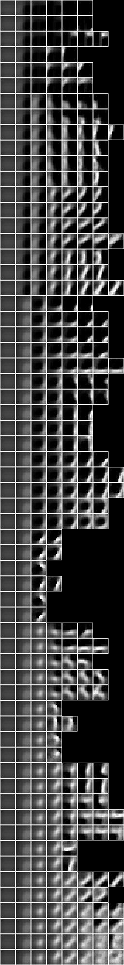
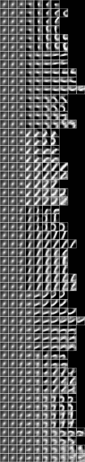
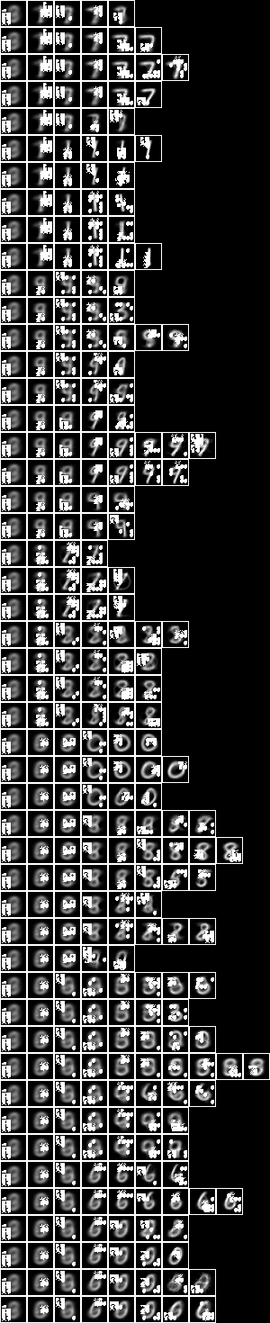
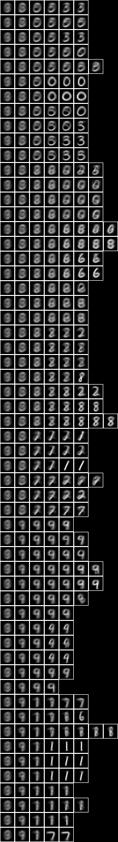
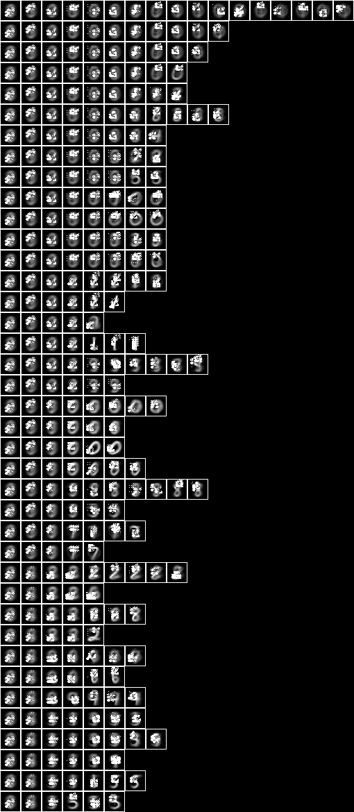
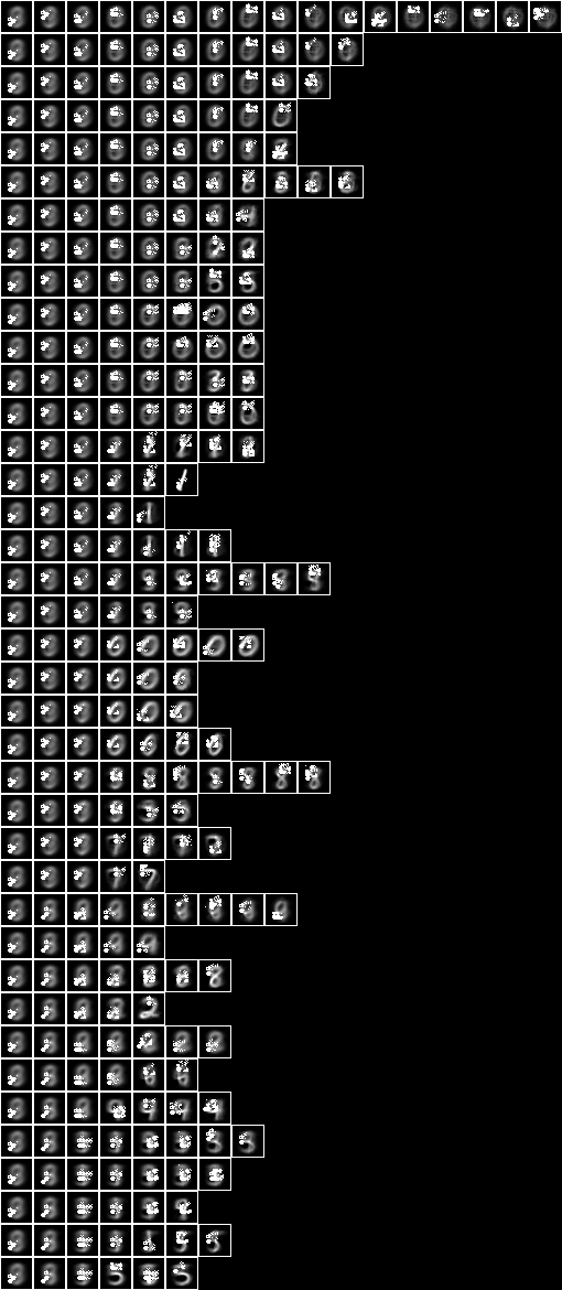
Below is an image of the fud decomposition, and adjacent is an image of the fud underlying superimposed on the slices,
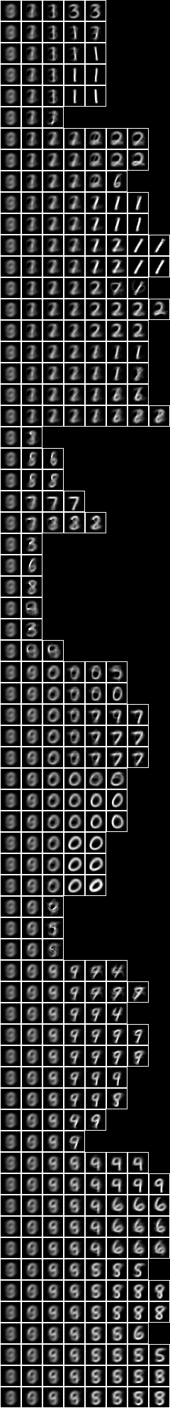
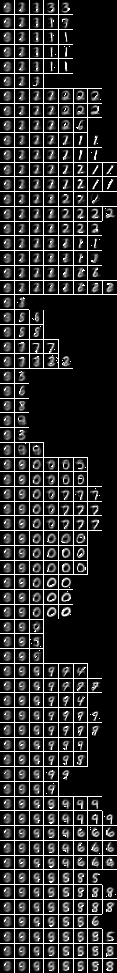
A magnified image of the fud underlying superimposed on the averaged slice, can be seen at Model 35.
pp = treesPaths(hrmult(uu1,df,hr))

def fid(ff):
    return variablesVariableFud(fder(ff)[0])

rpln([[fid(ff) for ((_,ff),_) in ll] for ll in pp])
# [1, 4, 12, 31, 77]
# [1, 4, 12, 47, 99]
# [1, 4, 12, 47, 103]
# [1, 4, 12, 37, 85]
# [1, 4, 12, 37, 96]
# ...
# [1, 4, 5, 8, 14, 24, 46, 66]
# [1, 94]
# [1, 29, 98]
# [1, 29, 49]
# 1, 21, 51, 105]
# [1, 21, 41, 76, 120]
# [1, 69]
# ...
# [1, 2, 3, 6, 10, 15, 34, 107]
# [1, 2, 3, 6, 10, 15, 34, 52]
# [1, 2, 3, 6, 10, 15, 45, 80]

rpln([[hrsize(hr) for (_,hr) in ll] for ll in pp])
# [7500, 2259, 759, 211, 83]
# [7500, 2259, 759, 194, 95]
# [7500, 2259, 759, 194, 99]
# [7500, 2259, 759, 220, 106]
# [7500, 2259, 759, 220, 95]
# ...
# [7500, 2259, 1121, 662, 397, 179, 77, 64]
# [7500, 64]
# [7500, 212, 96]
# [7500, 212, 115]
# [7500, 300, 139, 70]
# [7500, 300, 158, 67, 46]
# [7500, 65]
# ...
# [7500, 3718, 2155, 1440, 743, 544, 212, 81]
# [7500, 3718, 2155, 1440, 743, 544, 212, 128]
# [7500, 3718, 2155, 1440, 743, 544, 169, 76]
We can see that the paths vary in length from two fuds to eight fuds. The paths of length two have small leaf off-diagonal slices and often seem to contain mixtures of odd cases. Longer paths tend to group more regular and recognisable digits. These paths successively resolve more and more details, such as the obliqueness of ones or the roundness of zeroes. Note that the model does not pay much attention to label alignments. More ‘complicated’ digits, such as fours or fives are neglected in favour of ‘simpler’ digits such as ones and zeroes.
The underlying tuple of the root slice is $\mathrm{und}(F)$, where $((\cdot,F),\cdot) = P_{1,1}$,
((_,ff),hrs) = pp[0][0]

fund(ff)
# {<10,11>, <10,12>, <11,10>, <11,11>, <11,12>, <12,9>, <12,10>, <12,11>, <13,9>, <13,10>, <13,11>, <14,9>, <14,10>, <15,9>}

bmwrite(file,bmborder(1,bmmax(hrbm(28,3,2,hrhrred(hrs,vvk)),0,0,hrbm(28,3,2,qqhr(2,uu,vvk,fund(ff))))))

It is similar to that of the 15-fud model, above. The first child slice of the second column has size 2259. It resembles the corresponding slice of size 2584 in the 15-fud model. It has quite a different underlying tuple, though,
((_,ff),hrs) = pp[0][1]

fund(ff)
# {<18,12>, <18,13>, <19,11>, <19,12>, <19,13>, <20,10>, <20,11>, <20,12>, <20,13>, <21,10>, <21,11>, <21,12>, <21,13>}

bmwrite(file,bmborder(1,bmmax(hrbm(28,3,2,hrhrred(hrs,vvk)),0,0,hrbm(28,3,2,qqhr(2,uu,vvk,fund(ff))))))

The 15-fud model 2 resembles the near-root parts of 127-fud model 35.
Now let us query the model with a sample event to see how it is being classified. First, consider the fud decomposition fud, $F = D^{\mathrm{F}}$, (see Practicable fud decomposition fud),
ff = dfnul(uu1,df,1)

len(fvars(ff))
5597

len(fder(ff))
1316

list(fder(ff))[:20]
# [<<1,n>,1>, <<1,n>,2>, <<1,n>,3>, <<1,n>,4>, <<1,n>,5>, <<1,n>,6>, <<1,n>,7>, <<1,n>,8>, <<1,n>,9>, <<1,n>,10>, <<1,n>,11>, <<2,n>,1>, <<2,n>,2>, <<2,n>,3>, <<2,n>,4>, <<2,n>,5>, <<2,n>,6>, <<2,n>,7>, <<2,n>,8>, <<2,n>,9>]
Now apply the model to the sample history, $A_{\mathrm{b}} = A * \prod \mathrm{his}(F)$,
uu2 = uunion(uu,fsys(ff))

hrb = hrfmul(uu2,ff,hr)

hrsize(hrb)
7500

len(hrvars(hrb))
5894
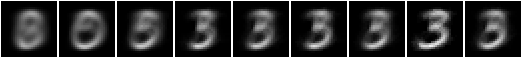
Choose, for example, the first event $Q = \{S\}^{\mathrm{U}}$, where $S \in (A\%V_{\mathrm{k}})^{\mathrm{S}}$,
hrq = hrev([0],hrhrred(hr,vvk))

bmwrite(file,bmborder(1,hrbm(28,2,2,hrq)))

Now find the leaf slice of the query, $A_{\mathrm{c}} = A_{\mathrm{b}} * (Q * F^{\mathrm{T}})$,
hrc = hrhrsel(hrb,hrhrred(hrfmul(uu2,ff,hrq),fder(ff)))

hrsize(hrc)
53

bmwrite(file,bmborder(1,hrbm(28,2,2,hrhrred(hrc,vvk))))

Here are the first 20 slice events, $A_{\mathrm{c}}~\%~V_{\mathrm{k}}$,
hrc1 = hrhrred(hrc,vvk)

bmwrite(file,bmhstack([bmborder(1,hrbm(28,1,2,hrev([i],hrc1))) for i in range(min(20,hrsize(hrc1)))]))

The label variable is, $A_{\mathrm{c}}~\%~V_{\mathrm{l}}$,
rpln(aall(hhaa(hrhh(uu1,hrhrred(hrc,vvl)))))
# ({(digit, 1)}, 4 % 1)
# ({(digit, 3)}, 5 % 1)
# ({(digit, 4)}, 1 % 1)
# ({(digit, 5)}, 29 % 1)
# ({(digit, 8)}, 11 % 1)
# ({(digit, 9)}, 3 % 1)
The modal label is five, but the slice also contains eights and some other similar looking digits.
Now let us see how the slice was chosen. Here are the slices and their underlying for each non-null derived variable state, \[ \{A_{\mathrm{b}} * \{\{(w,u)\}\}^{\mathrm{U}}~\%~\{w\} : (S,\cdot) \in A_{\mathrm{c}}~\%~\mathrm{der}(F),~(w,u) \in S,~u \neq \mathrm{null}\} \]
ll = [(w,u) for (ss,_) in aall(hhaa(hrhh(uu2,hrhrred(hrc,fder(ff))))) for (w,u) in ssll(ss) if u != ValStr("null")]

hrb1 = hrhrred(hrb,vvk|sset([w for (w,u) in ll]))

rpln([hhaa(hrhh(uu2,hrhrred(hrhrsel(hrb1,aahr(uu2,rr)),vars(rr)))) for (w,u) in ll for rr in [single(llss([(w,u)]),1)]])
# {({(<<1,n>,1>, 0)}, 3252 % 1)}
# {({(<<1,n>,2>, 0)}, 3002 % 1)}
# {({(<<1,n>,3>, 0)}, 3247 % 1)}
# {({(<<1,n>,4>, 0)}, 2864 % 1)}
# {({(<<1,n>,5>, 0)}, 3042 % 1)}
# {({(<<1,n>,6>, 1)}, 4731 % 1)}
# {({(<<1,n>,7>, 0)}, 3021 % 1)}
# {({(<<1,n>,8>, 0)}, 2943 % 1)}
# {({(<<1,n>,9>, 0)}, 2814 % 1)}
# {({(<<1,n>,10>, 0)}, 3267 % 1)}
# {({(<<1,n>,11>, 1)}, 4662 % 1)}
# {({(<<29,n>,1>, 1)}, 115 % 1)}
# {({(<<29,n>,2>, 1)}, 115 % 1)}
# {({(<<29,n>,3>, 1)}, 115 % 1)}
# {({(<<29,n>,4>, 1)}, 115 % 1)}
# {({(<<29,n>,5>, 1)}, 115 % 1)}
# {({(<<29,n>,6>, 1)}, 115 % 1)}
# {({(<<29,n>,7>, 1)}, 116 % 1)}
# {({(<<29,n>,8>, 1)}, 116 % 1)}
# {({(<<29,n>,9>, 1)}, 116 % 1)}
# {({(<<29,n>,10>, 1)}, 116 % 1)}
# {({(<<29,n>,11>, 1)}, 116 % 1)}
# {({(<<49,n>,1>, 0)}, 53 % 1)}
# {({(<<49,n>,2>, 0)}, 55 % 1)}
# {({(<<49,n>,3>, 0)}, 58 % 1)}
# {({(<<49,n>,4>, 0)}, 53 % 1)}
# {({(<<49,n>,5>, 0)}, 57 % 1)}
# {({(<<49,n>,6>, 0)}, 53 % 1)}
# {({(<<49,n>,7>, 0)}, 54 % 1)}
# {({(<<49,n>,8>, 0)}, 54 % 1)}
# {({(<<49,n>,9>, 0)}, 55 % 1)}

bmwrite(file,bmhstack([bmborder(1,hrbm(28,1,2,hrhrred(hrhrsel(hrb1,aahr(uu2,rr)),vvk))) for (w,u) in ll for rr in [single(llss([(w,u)]),1)]]))

bmwrite(file,bmhstack([bmborder(1,hrbm(28,1,2,qqhr(2,uu,vvk,fund(fdep(ff,sset([w])))))) for (w,u) in ll]))


In this case, we can see that there are only three fuds in the decomposition path.
Now let us repeat the same analysis for the next event,
hrq = hrev([1],hrhrred(hr,vvk))

bmwrite(file,bmborder(1,hrbm(28,2,2,hrq)))

Now find the leaf slice of the query,
hrc = hrhrsel(hrb,hrhrred(hrfmul(uu2,ff,hrq),fder(ff)))

hrsize(hrc)
11

bmwrite(file,bmborder(1,hrbm(28,2,2,hrhrred(hrc,vvk))))

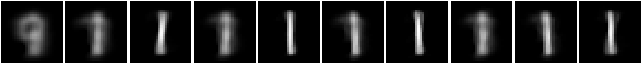
Here are the slice events,
hrc1 = hrhrred(hrc,vvk)

bmwrite(file,bmhstack([bmborder(1,hrbm(28,1,2,hrev([i],hrc1))) for i in range(min(20,hrsize(hrc1)))]))

The label variable is,
rpln(aall(hhaa(hrhh(uu1,hrhrred(hrc,vvl)))))
({(digit, 1)}, 11 % 1)
In this case the entire slice consists of ones.
Here are the slices and their underlying for each non-null derived variable state,
ll = [(w,u) for (ss,_) in aall(hhaa(hrhh(uu2,hrhrred(hrc,fder(ff))))) for (w,u) in ssll(ss) if u != ValStr("null")]

hrb1 = hrhrred(hrb,vvk|sset([w for (w,u) in ll]))

rpln([hhaa(hrhh(uu2,hrhrred(hrhrsel(hrb1,aahr(uu2,rr)),vars(rr)))) for (w,u) in ll for rr in [single(llss([(w,u)]),1)]])
# {({(<<1,n>,1>, 0)}, 3252 % 1)}
# {({(<<1,n>,2>, 0)}, 3002 % 1)}
# {({(<<1,n>,3>, 0)}, 3247 % 1)}
# {({(<<1,n>,4>, 0)}, 2864 % 1)}
# {({(<<1,n>,5>, 0)}, 3042 % 1)}
# {({(<<1,n>,6>, 0)}, 2769 % 1)}
# {({(<<1,n>,7>, 0)}, 3021 % 1)}
# {({(<<1,n>,8>, 0)}, 2943 % 1)}
# {({(<<1,n>,9>, 0)}, 2814 % 1)}
# {({(<<1,n>,10>, 0)}, 3267 % 1)}
# {({(<<1,n>,11>, 0)}, 2838 % 1)}
# {({(<<4,n>,1>, 0)}, 1002 % 1)}
# {({(<<4,n>,2>, 0)}, 894 % 1)}
# {({(<<4,n>,3>, 0)}, 963 % 1)}
# {({(<<4,n>,4>, 0)}, 963 % 1)}
# {({(<<4,n>,5>, 0)}, 875 % 1)}
# {({(<<4,n>,6>, 0)}, 917 % 1)}
# {({(<<4,n>,7>, 0)}, 914 % 1)}
# {({(<<4,n>,8>, 0)}, 888 % 1)}
# {({(<<4,n>,9>, 0)}, 926 % 1)}
# {({(<<4,n>,10>, 0)}, 976 % 1)}
# {({(<<4,n>,11>, 0)}, 1034 % 1)}
# {({(<<12,n>,1>, 1)}, 493 % 1)}
# {({(<<12,n>,2>, 1)}, 498 % 1)}
# {({(<<12,n>,3>, 1)}, 504 % 1)}
# {({(<<12,n>,4>, 1)}, 320 % 1)}
# {({(<<12,n>,5>, 1)}, 281 % 1)}
# {({(<<12,n>,6>, 1)}, 288 % 1)}
# {({(<<12,n>,7>, 1)}, 472 % 1)}
# {({(<<12,n>,8>, 1)}, 545 % 1)}
# {({(<<12,n>,9>, 1)}, 512 % 1)}
# {({(<<47,n>,1>, 1)}, 99 % 1)}
# {({(<<47,n>,2>, 1)}, 99 % 1)}
# {({(<<47,n>,3>, 1)}, 99 % 1)}
# {({(<<47,n>,4>, 1)}, 99 % 1)}
# {({(<<47,n>,5>, 1)}, 99 % 1)}
# {({(<<47,n>,6>, 1)}, 99 % 1)}
# {({(<<47,n>,7>, 1)}, 99 % 1)}
# {({(<<47,n>,8>, 1)}, 99 % 1)}
# {({(<<47,n>,9>, 1)}, 99 % 1)}
# {({(<<47,n>,10>, 1)}, 99 % 1)}
# {({(<<47,n>,11>, 1)}, 99 % 1)}
# {({(<<103,n>,1>, 0)}, 37 % 1)}
# {({(<<103,n>,2>, 0)}, 37 % 1)}
# {({(<<103,n>,3>, 1)}, 73 % 1)}
# {({(<<103,n>,4>, 1)}, 73 % 1)}
# {({(<<103,n>,5>, 1)}, 77 % 1)}
# {({(<<103,n>,6>, 0)}, 39 % 1)}
# {({(<<103,n>,7>, 1)}, 73 % 1)}
# {({(<<103,n>,8>, 1)}, 73 % 1)}
# {({(<<103,n>,9>, 0)}, 39 % 1)}
# {({(<<103,n>,10>, 1)}, 73 % 1)}
# {({(<<103,n>,11>, 1)}, 77 % 1)}

bmwrite(file,bmhstack([bmborder(1,hrbm(28,1,2,hrhrred(hrhrsel(hrb1,aahr(uu2,rr)),vvk))) for (w,u) in ll for rr in [single(llss([(w,u)]),1)]]))

bmwrite(file,bmhstack([bmborder(1,hrbm(28,1,2,qqhr(2,uu,vvk,fund(fdep(ff,sset([w])))))) for (w,u) in ll]))


Now there are five fuds in the decomposition path, so the classification is more gradual.
Averaged pixels
Now consider a 127-fud induced model of the 60,000 events of the training sample NIST_model34.json which is induced by NIST_engine34.py, (see Model 34).
We shall analyse it with the 7,500 events subset of the sample,
from NISTDev import *

(uu,hrtr) = nistTrainBucketedAveragedIO(8,9,0)

digit = VarStr("digit")
vv = uvars(uu)
vvl = sset([digit])
vvk = vv - vvl

hr = hrev([i for i in range(hrsize(hrtr)) if i % 8 == 0],hrtr)

hrsize(hr)
7500

df = dfIO('./NIST_model34.json')

uu1 = uunion(uu,fsys(dfff(df)))

len(dfund(df))
70

len(fvars(dfff(df)))
4553

(wmax,lmax,xmax,omax,bmax,mmax,umax,pmax,fmax,mult,seed) = (2**11, 8, 2**10, 30, (30*3), 3, 2**8, 1, 127, 1, 5)

summation(mult,seed,uu1,df,hr)
# (79321.15706532392, 37342.43322059577)
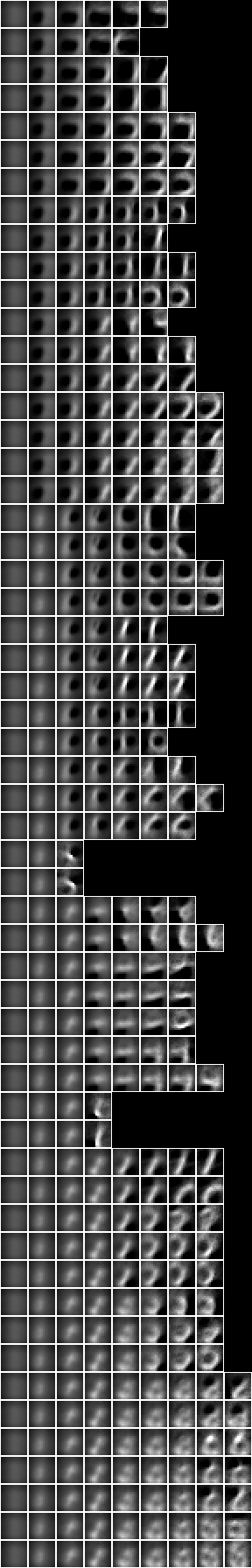
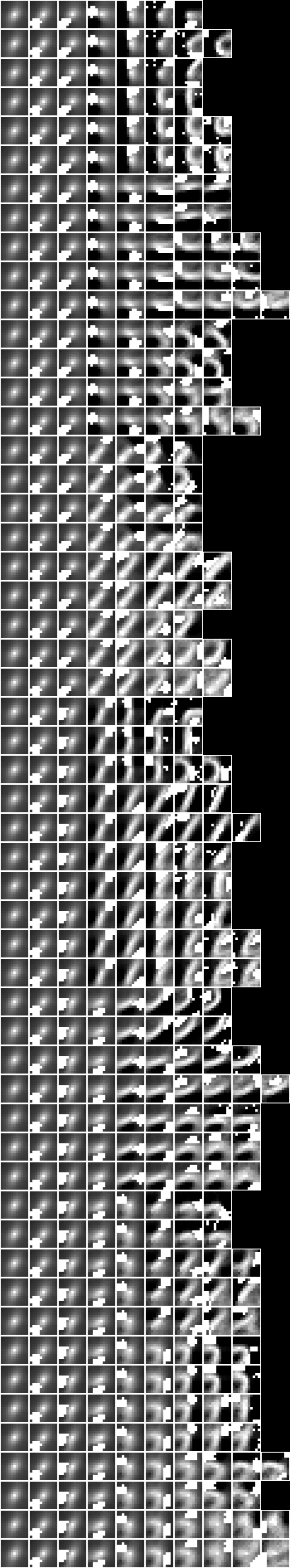
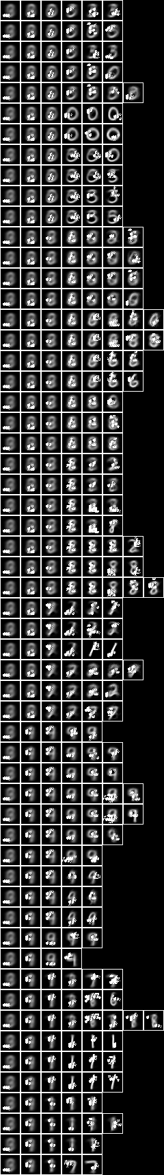
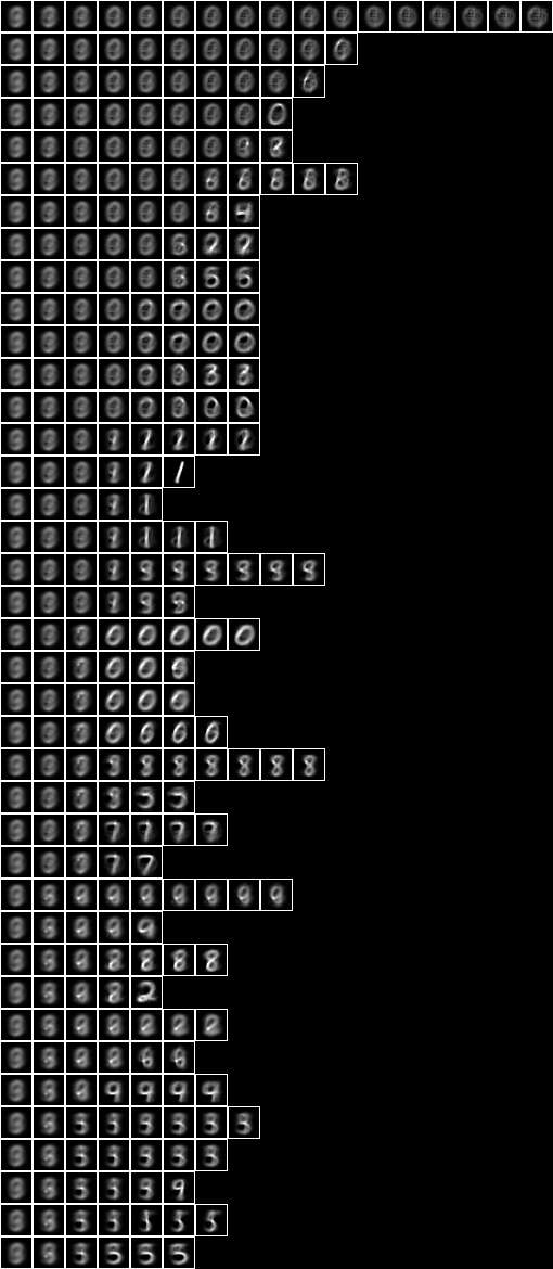
Below is an image of the fud decomposition, and adjacent is an image of the fud underlying superimposed on the slices,

A magnified image of the fud underlying superimposed on the averaged slice, can be seen at Model 34.
pp = treesPaths(hrmult(uu1,df,hr))

rpln([[hrsize(hr) for (_,hr) in ll] for ll in pp])
# [7500, 1978, 732, 197, 82]
# [7500, 1978, 732, 197, 69]
# [7500, 1978, 732, 197, 26, 14]
# ...
# [7500, 1978, 1208, 581, 395, 305, 142, 49, 11]
# [7500, 1978, 1208, 581, 395, 30]
# [7500, 1978, 1208, 581, 125]
# ...
# [7500, 394, 319, 60, 37]
# [7500, 99, 89]
# [7500, 32]
# [7500, 24, 23]
# [7500, 57]
# [7500, 51]
# [7500, 32]
# [7500, 74, 69]
# ...
# [7500, 4273, 1674, 304, 114, 64]
# [7500, 4273, 1674, 304, 29]
# [7500, 4273, 158, 136]
Similarly to the all-pixels case above, we can see that the paths vary in length from two fuds to nine fuds. Here the clusters of the underlying tuples are spread over more of the digit, and so the classification is less localised. The longer paths divide less according to style and more according to label, than the all-pixels model.
The underlying tuple of the root slice is,
((_,ff),hrs) = pp[0][0]

fund(ff)
# {<3,7>, <4,3>, <4,4>, <4,8>, <5,3>, <5,7>, <5,8>, <6,3>, <6,7>, <6,8>, <7,3>, <7,7>, <7,8>}

bmwrite(file,bmborder(1,bmmax(hrbm(9,(3*2),8,hrhrred(hrs,vvk)),0,0,hrbm(9,(3*2),8,qqhr(8,uu,vvk,fund(ff))))))

It is similar to the first tuple of the investigation of the properties of the sample using the tupler, above.
Square regions of 10x10 pixels
Now consider a 127-fud induced model of square regions of 10x10 pixels chosen randomly from the images of the 60,000 events of the training sample NIST_model6.json which is induced by NIST_engine6.py. (See Model induction.)
We shall analyse it with the 7,500 events subset of the sample,
from NISTDev import *

(uu,hrtr) = nistTrainBucketedRegionRandomIO(2,10,17)

digit = VarStr("digit")
vv = uvars(uu)
vvl = sset([digit])
vvk = vv - vvl

hr = hrev([i for i in range(hrsize(hrtr)) if i % 8 == 0],hrtr)

hrsize(hr)
7500

df = dfIO('./NIST_model6.json')

uu1 = uunion(uu,fsys(dfff(df)))

len(dfund(df))
100

len(fvars(dfff(df)))
3842

(wmax,lmax,xmax,omax,bmax,mmax,umax,pmax,fmax,mult,seed) = (2**11, 8, 2**10, 30, (30*3), 3, 2**8, 1, 127, 1, 5)

summation(mult,seed,uu1,df,hr)
# (158224.09183189203, 78504.46852158802)
Imaging the fud decomposition,
Square regions of 15x15 pixels
Now consider a 127-fud induced model of square regions of 15x15 pixels chosen randomly from the images of the 60,000 events of the training sample NIST_model21.json which is induced by NIST_engine21.py. (See Model induction.)
We shall analyse it with the 7,500 events subset of the sample,
from NISTDev import *

(uu,hrtr) = nistTrainBucketedRegionRandomIO(2,15,17)

digit = VarStr("digit")
vv = uvars(uu)
vvl = sset([digit])
vvk = vv - vvl

hr = hrev([i for i in range(hrsize(hrtr)) if i % 8 == 0],hrtr)

hrsize(hr)
7500

df = dfIO('./NIST_model21.json')

uu1 = uunion(uu,fsys(dfff(df)))

len(dfund(df))
225

len(fvars(dfff(df)))
4082

(wmax,lmax,xmax,omax,bmax,mmax,umax,pmax,fmax,mult,seed) = (2**11, 8, 2**10, 30, (30*3), 3, 2**8, 1, 127, 1, 5)

summation(mult,seed,uu1,df,hr)
# (195132.9636225562, 97210.92592647046)
Imaging the fud decomposition,
Centred square regions of 11x11 pixels
Now consider a 127-fud induced model applied to centred square regions of 11x11 pixels chosen randomly from the images of the 60,000 events of the training sample NIST_model10.json which is induced by NIST_engine10.py. (See Model induction.)
We shall analyse it with the 7,500 events subset of the sample,
from NISTDev import *

(uu,hrtr) = nistTrainBucketedRegionRandomIO(2,11,17)

digit = VarStr("digit")
vv = uvars(uu)
vvl = sset([digit])
vvk = vv - vvl

hr = hrev([i for i in range(hrsize(hrtr)) if i % 8 == 0],hrtr)

hrsize(hr)
7500

df = dfIO('./NIST_model10.json')

uu1 = uunion(uu,fsys(dfff(df)))

len(dfund(df))
121

len(fvars(dfff(df)))
3711

(wmax,lmax,xmax,omax,bmax,mmax,umax,pmax,fmax,mult,seed) = (2**11, 8, 2**10, 30, (30*3), 3, 2**8, 1, 127, 1, 5)

summation(mult,seed,uu1,df,hr)
(47814.604663722406, 23823.320394470335)
Imaging the fud decomposition,
Two level over 10x10 regions
Let us consider a two level model which consists of 5x5 frames of square regions of 10x10 pixels.
First we will reduce the underlying 127-fud decomposition $D$ so that the resultant decomposition fud does not make an excessively large level substrate. The reduced decomposition is a sub-model constructed by selecting only one derived variable and its dependents in each fud of the decomposition. In the case where the fuds are highly diagonalised this usually leads to a reasonable approximation of the model. Let us examine this reduced decomposition $D_{\mathrm{r}}$,
from NISTDev import *

(uu,hrtr) = nistTrainBucketedRegionRandomIO(2,10,17)

digit = VarStr("digit")
vv = uvars(uu)
vvl = sset([digit])
vvk = vv - vvl

hr = hrev([i for i in range(hrsize(hrtr)) if i % 8 == 0],hrtr)

hrsize(hr)
7500

df = dfIO('./NIST_model6.json')

uu1 = uunion(uu,fsys(dfff(df)))

len(dfund(df))
100

len(fvars(dfff(df)))
3842

dfred = systemsDecompFudsHistoryRepasDecompFudReduced

dfr = dfred(uu1,df,hr)

len(dfund(dfr))
100

len(fder(dfff(dfr)))
126

len(fvars(dfff(dfr)))
634
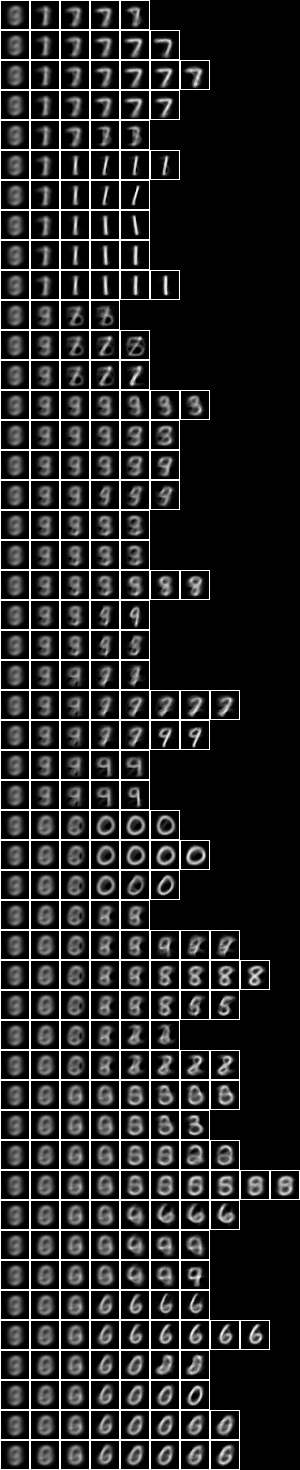
Imaging the reduced fud decomposition,
pp = treesPaths(hrmult(uu1,dfr,hr))

bmwrite(file,ppbm2(uu,vvk,10,3,2,pp))
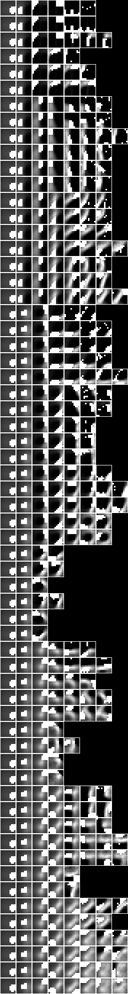
The reduced fud decomposition on the left may be compared to the original fud decomposition on the right,
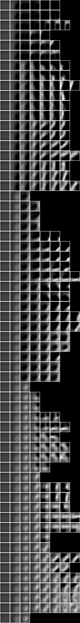
The images are similar in spite of the reduction.
Having reduced the level 1 model we can then make 5x5 copies of it to cover the 28x28 pixels of the sample substrate - see Model induction. The model NIST_model24.json is induced by NIST_engine24.py.
We shall analyse it with the 7,500 events subset of the sample. Note that these larger models require over 3GB memory to calculate the summation,
from NISTDev import *

(uu,hrtr) = nistTrainBucketedIO(2)

digit = VarStr("digit")
vv = uvars(uu)
vvl = sset([digit])
vvk = vv - vvl

hr = hrev([i for i in range(hrsize(hrtr)) if i % 8 == 0],hrtr)

hrsize(hr)
7500

df = dfIO('./NIST_model24.json')

uu1 = uunion(uu,fsys(dfff(df)))

len(dfund(df))
639

len(fvars(dfff(df)))
5966

(wmax,lmax,xmax,omax,bmax,mmax,umax,pmax,fmax,mult,seed) = (2**11, 8, 2**10, 30, (30*3), 3, 2**8, 1, 127, 1, 5)

summation(mult,seed,uu1,df,hr)
# (190022.26132400509, 89892.41155833867)
We can compare this 2-level model to the all pixels 1-level model,
summation mult seed uu1 df hr
# (132688.71288792725, 64806.344175194274)
The 2-level model is considerably more aligned.
Below is an image of the fud decomposition, and adjacent is an image of the fud underlying superimposed on the slices,
A magnified image of the fud underlying superimposed on the averaged slice, can be seen at Model 24.
We can see that the fud underlying clusters are larger in general than for the 1-level model. The paths vary in length from four fuds to ten fuds. The tree is more uniform than for the 1-level model. That is, there are fewer effective off-diagonal states.
Let us reduce the 2-level model, $D$, to make it more managable, $D_{\mathrm{r}}$,
dfr = dfred(uu1,df,hr)

len(dfund(dfr))
623

len(fder(dfff(dfr)))
127

len(fvars(dfff(dfr)))
3310
Let us examine the slices, $P = \mathrm{paths}(A * D_{\mathrm{r}})$,
def variablesVariableFud(x):
    if isinstance(x, VarPair):
        (w,_) = x._rep
        if isinstance(w, VarPair):
            (u,_) = w._rep
            if isinstance(u, VarPair):
                (f,_) = u._rep
            return f
    return VarInt(0)

def fid(ff):
    return variablesVariableFud(fder(ff)[0])

pp = treesPaths(hrmult(uu1,dfr,hr))

rpln([(i,[fid(ff) for ((_,ff),_) in ll]) for (i,ll) in enumerate(pp)])
# (0, [1, 6, 12, 20, 56])
# (1, [1, 6, 12, 20, 30, 112])
# (2, [1, 6, 12, 20, 30, 71, 125])
# ...
# (6, [1, 6, 17, 46, 127])
# (7, [1, 6, 17, 32, 110])
# (8, [1, 6, 17, 32, 115])
# ...
# (46, [1, 2, 3, 9, 19, 27, 94])
# (47, [1, 2, 3, 9, 19, 27, 88, 121])
# (48, [1, 2, 3, 9, 19, 27, 63, 86])

rpln([(i,[hrsize(hr) for (_,hr) in ll]) for (i,ll) in enumerate(pp)])
# (0, [7500, 1653, 860, 546, 247])
# (1, [7500, 1653, 860, 546, 299, 98])
# (2, [7500, 1653, 860, 546, 299, 201, 97])
# ...
# (6, [7500, 1653, 793, 302, 91])
# (7, [7500, 1653, 793, 491, 159])
# (8, [7500, 1653, 793, 491, 332])
# ...
# (46, [7500, 3499, 2094, 626, 294, 229, 75])
# (47, [7500, 3499, 2094, 626, 294, 229, 154, 103])
# (48, [7500, 3499, 2094, 626, 294, 229, 154, 108])
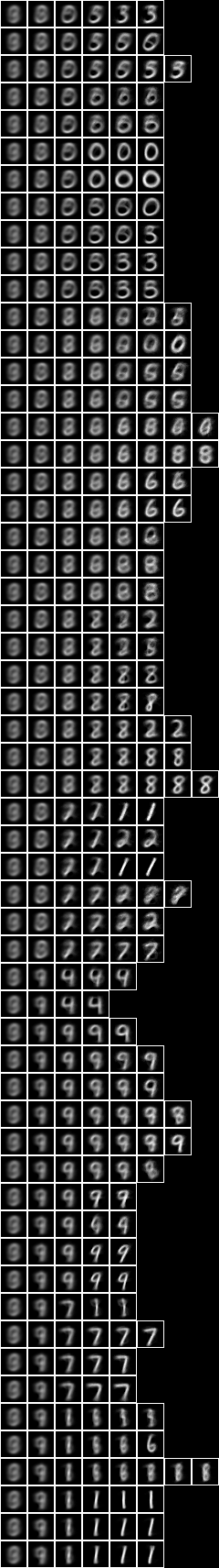
Imaging the reduced decomposition slices,
file = "NIST.bmp"

bmwrite(file,ppbm2(uu,vvk,28,1,2,pp))

bmwrite(file,ppbm(uu,vvk,28,1,2,pp))
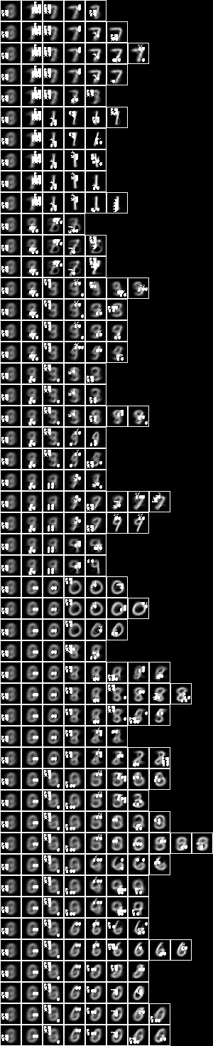
Again, the reduced decomposition is similar to the original decomposition.
The underlying tuple of the root slice is $\mathrm{und}(F)$, where $((\cdot,F),\cdot) = P_{1,1}$,
((_,ff),hrs) = pp[0][0]

len(fund(ff))
69

bmwrite(file,bmborder(1,bmmax(hrbm(28,3,2,hrhrred(hrs,vvk)),0,0,hrbm(28,3,2,qqhr(2,uu,vvk,fund(ff))))))

We can see that the root slice depends on an underlying cluster that is larger than the corresponding cluster for the root slice in the 1-level model. It is also in a different location.
The first child slice of the second column has size 1653,
((_,ff),hrs) = pp[0][1]

len(fund(ff))
164

bmwrite(file,bmborder(1,bmmax(hrbm(28,3,2,hrhrred(hrs,vvk)),0,0,hrbm(28,3,2,qqhr(2,uu,vvk,fund(ff))))))

Again, we can see that the root slice depends on a larger cluster of the substrate than in the 1-level model.
Now let us query the model with a sample event to see how it is being classified. First, consider the fud decomposition fud, $F = D_{\mathrm{r}}^{\mathrm{F}}$, (see Practicable fud decomposition fud),
ff = dfnul(uu1,dfr,2)

len(fvars(ff))
3685

len(fder(ff))
127

list(fder(ff))[:5]
# [<<<1,1>,n2>,1>, <<<2,1>,n2>,1>, <<<3,1>,n2>,1>, <<<4,1>,n2>,1>, <<<5,1>,n2>,1>]
Now apply the model to the sample history, $A_{\mathrm{b}} = A * \prod \mathrm{his}(F)$,
uu2 = uunion(uu,fsys(ff))

hrb = hrfmul(uu2,ff,hr)

hrsize(hrb)
7500

len(hrvars(hrb))
3847
Choose, for example, the first event $Q = \{S\}^{\mathrm{U}}$, where $S \in (A\%V_{\mathrm{k}})^{\mathrm{S}}$,
hrq = hrev([0],hrhrred(hr,vvk))

bmwrite(file,bmborder(1,hrbm(28,2,2,hrq)))
Now find the leaf slice of the query, $A_{\mathrm{c}} = A_{\mathrm{b}} * (Q * F^{\mathrm{T}})$,
hrc = hrhrsel(hrb,hrhrred(hrfmul(uu2,ff,hrq),fder(ff)))

hrsize(hrc)
108

bmwrite(file,bmborder(1,hrbm(28,2,2,hrhrred(hrc,vvk))))

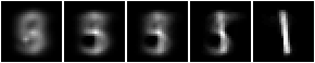
Here are the first 20 slice events, $A_{\mathrm{c}}~\%~V_{\mathrm{k}}$,
hrc1 = hrhrred(hrc,vvk)

bmwrite(file,bmhstack([bmborder(1,hrbm(28,1,2,hrev([i],hrc1))) for i in range(min(20,hrsize(hrc1)))]))

The label variable is, $A_{\mathrm{c}}~\%~V_{\mathrm{l}}$,
rpln(aall(hhaa(hrhh(uu1,hrhrred(hrc,vvl)))))
# ({(digit, 1)}, 3 % 1)
# ({(digit, 2)}, 8 % 1)
# ({(digit, 3)}, 12 % 1)
# ({(digit, 4)}, 3 % 1)
# ({(digit, 5)}, 4 % 1)
# ({(digit, 6)}, 2 % 1)
# ({(digit, 7)}, 29 % 1)
# ({(digit, 8)}, 43 % 1)
# ({(digit, 9)}, 4 % 1)
The modal label is eight and there are only a few fives, but some of the slice digits look similar to the five.
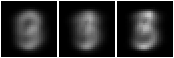
Now let us see how the event was chosen. Here are the slices and their underlying for each non-null derived variable state, \[ \{A_{\mathrm{b}} * \{\{(w,u)\}\}^{\mathrm{U}}~\%~\{w\} : (S,\cdot) \in Q * F^{\mathrm{T}},~(w,u) \in S,~u \neq \mathrm{null}\} \]
hrqb = hrfmul(uu2,ff,hrq)

ll = [(w,u) for (ss,_) in aall(hhaa(hrhh(uu2,hrhrred(hrqb,fder(ff))))) for (w,u) in ssll(ss) if u != ValStr("null")]

hrb1 = hrhrred(hrb,vvk|sset([w for (w,u) in ll]))

rpln([hhaa(hrhh(uu2,hrhrred(hrhrsel(hrb1,aahr(uu2,rr)),vars(rr)))) for (w,u) in ll for rr in [single(llss([(w,u)]),1)]])
# {({(<<<1,1>,n2>,1>, 0)}, 1653 % 1)}
# {({(<<<6,1>,n2>,1>, 0)}, 860 % 1)}
# {({(<<<12,1>,n2>,1>, 0)}, 546 % 1)}
# {({(<<<20,1>,n2>,1>, 0)}, 247 % 1)}
# {({(<<<56,1>,n2>,1>, 0)}, 108 % 1)}

bmwrite(file,bmhstack([bmborder(1,hrbm(28,2,2,hrhrred(hrhrsel(hrb1,aahr(uu2,rr)),vvk))) for (w,u) in ll for rr in [single(llss([(w,u)]),1)]]))

bmwrite(file,bmhstack([bmborder(1,hrbm(28,2,2,qqhr(2,uu,vvk,fund(fdep(ff,sset([w])))))) for (w,u) in ll]))

Note that we are considering the reduced decomposition, $D_{\mathrm{r}}$, which can be indistinct, so the non-null derived variables do not necessarily correspond to just one path of the original decomposition, $D$. In this case they do correspond to one path,
# (0, [1, 6, 12, 20, 56])
# ...

bmwrite(file,bmhstack([bmborder(1,hrbm(28,1,2,hrhrred(hrs,vvk))) for (_,hrs) in pp[0]]))
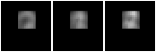
Let us examine the level 1 nullable derived variables of the central region at (10;10),
def islevnull(x):
    if isinstance(x, VarPair):
        (w,c) = x._rep
        if isinstance(w, VarPair) and isinstance(c, VarStr) and c._rep == "(10;10)":
            (u,_) = w._rep
            if isinstance(u, VarPair):
                (_,g) = u._rep
                if isinstance(g, VarStr) and g._rep == "n":
                    return True
    return False

len([w for w in fvars(ff) if islevnull(w)])
8

ll = list(sset([(w,u) for (ss,_) in aall(hhaa(hrhh(uu2,hrhrred(hrqb,sset([w for w in fvars(ff) if islevnull(w)]))))) for (w,u) in ssll(ss) if u != ValStr("null")]))

hrb1 = hrhrred(hrb,vvk|sset([w for (w,u) in ll]))

rpln([hhaa(hrhh(uu2,hrhrred(hrhrsel(hrb1,aahr(uu2,rr)),vars(rr)))) for (w,u) in ll for rr in [single(llss([(w,u)]),1)]])
# {({(<<<<<1,1>,0>,n>,1>,(10;10)>, 1)}, 6550 % 1)}
# {({(<<<<<1,2>,0>,n>,1>,(10;10)>, 1)}, 5190 % 1)}
# {({(<<<<<1,86>,0>,n>,1>,(10;10)>, 0)}, 1999 % 1)}
# {({(<<<<<1,96>,0>,n>,1>,(10;10)>, 1)}, 2130 % 1)}

bmwrite(file,bmhstack([bmborder(1,hrbm(28,2,2,hrhrred(hrhrsel(hrb1,aahr(uu2,rr)),vvk))) for (w,u) in ll for rr in [single(llss([(w,u)]),1)]]))

bmmask = bminsert(bmempty(28*2,28*2),10*2-1,10*2-1,bmfull(10*2,10*2))

bmwrite(file,bmhstack([bmborder(1,bmmin(bmmask,0,0,hrbm(28,2,2,hrhrred(hrhrsel(hrb1,aahr(uu2,rr)),vvk)))) for (w,u) in ll for rr in [single(llss([(w,u)]),1)]]))

bmwrite(file,bmhstack([bmborder(1,hrbm(28,2,2,qqhr(2,uu,vvk,fund(fdep(ff,sset([w])))))) for (w,u) in ll]))

This frame detects the middle section of the five.
We can compare this region to the region, say, at (2;18),
def islevnull(x):
    if isinstance(x, VarPair):
        (w,c) = x._rep
        if isinstance(w, VarPair) and isinstance(c, VarStr) and c._rep == "(2;18)":
            (u,_) = w._rep
            if isinstance(u, VarPair):
                (_,g) = u._rep
                if isinstance(g, VarStr) and g._rep == "n":
                    return True
    return False

len([w for w in fvars(ff) if islevnull(w)])
2

ll = list(sset([(w,u) for (ss,_) in aall(hhaa(hrhh(uu2,hrhrred(hrqb,sset([w for w in fvars(ff) if islevnull(w)]))))) for (w,u) in ssll(ss) if u != ValStr("null")]))

hrb1 = hrhrred(hrb,vvk|sset([w for (w,u) in ll]))

rpln([hhaa(hrhh(uu2,hrhrred(hrhrsel(hrb1,aahr(uu2,rr)),vars(rr)))) for (w,u) in ll for rr in [single(llss([(w,u)]),1)]])
# {({(<<<<<1,1>,0>,n>,1>,(2;18)>, 0)}, 7059 % 1)}

bmwrite(file,bmhstack([bmborder(1,hrbm(28,2,2,hrhrred(hrhrsel(hrb1,aahr(uu2,rr)),vvk))) for (w,u) in ll for rr in [single(llss([(w,u)]),1)]]))

bmmask = bminsert(bmempty(28*2,28*2),2*2-1,18*2-1,bmfull(10*2,10*2))

bmwrite(file,bmhstack([bmborder(1,bmmin(bmmask,0,0,hrbm(28,2,2,hrhrred(hrhrsel(hrb1,aahr(uu2,rr)),vvk)))) for (w,u) in ll for rr in [single(llss([(w,u)]),1)]]))

bmwrite(file,bmhstack([bmborder(1,hrbm(28,2,2,qqhr(2,uu,vvk,fund(fdep(ff,sset([w])))))) for (w,u) in ll]))


This frame misses the top right tip of the five.
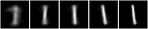
We can compare again to the region at (6;10),
def islevnull(x):
    if isinstance(x, VarPair):
        (w,c) = x._rep
        if isinstance(w, VarPair) and isinstance(c, VarStr) and c._rep == "(6;10)":
            (u,_) = w._rep
            if isinstance(u, VarPair):
                (_,g) = u._rep
                if isinstance(g, VarStr) and g._rep == "n":
                    return True
    return False

len([w for w in fvars(ff) if islevnull(w)])
6

ll = list(sset([(w,u) for (ss,_) in aall(hhaa(hrhh(uu2,hrhrred(hrqb,sset([w for w in fvars(ff) if islevnull(w)]))))) for (w,u) in ssll(ss) if u != ValStr("null")]))

hrb1 = hrhrred(hrb,vvk|sset([w for (w,u) in ll]))

rpln([hhaa(hrhh(uu2,hrhrred(hrhrsel(hrb1,aahr(uu2,rr)),vars(rr)))) for (w,u) in ll for rr in [single(llss([(w,u)]),1)]])
# {({(<<<<<1,1>,0>,n>,1>,(6;10)>, 1)}, 6457 % 1)}
# {({(<<<<<1,2>,0>,n>,1>,(6;10)>, 1)}, 4140 % 1)}
# {({(<<<<<1,69>,0>,n>,1>,(6;10)>, 1)}, 1929 % 1)}

bmwrite(file,bmhstack([bmborder(1,hrbm(28,2,2,hrhrred(hrhrsel(hrb1,aahr(uu2,rr)),vvk))) for (w,u) in ll for rr in [single(llss([(w,u)]),1)]]))

bmmask = bminsert(bmempty(28*2,28*2),6*2-1,10*2-1,bmfull(10*2,10*2))

bmwrite(file,bmhstack([bmborder(1,bmmin(bmmask,0,0,hrbm(28,2,2,hrhrred(hrhrsel(hrb1,aahr(uu2,rr)),vvk)))) for (w,u) in ll for rr in [single(llss([(w,u)]),1)]]))

bmwrite(file,bmhstack([bmborder(1,hrbm(28,2,2,qqhr(2,uu,vvk,fund(fdep(ff,sset([w])))))) for (w,u) in ll]))

This frame detects the top arc of the five.
Now let us repeat the same analysis for the next event,
hrq = hrev([1],hrhrred(hr,vvk))

bmwrite(file,bmborder(1,hrbm(28,2,2,hrq)))
Now find the leaf slice of the query,
hrc = hrhrsel(hrb,hrhrred(hrfmul(uu2,ff,hrq),fder(ff)))

hrsize(hrc)
75

bmwrite(file,bmborder(1,hrbm(28,2,2,hrhrred(hrc,vvk))))

Here are the first 20 slice events,
hrc1 = hrhrred(hrc,vvk)

bmwrite(file,bmhstack([bmborder(1,hrbm(28,1,2,hrev([i],hrc1))) for i in range(min(20,hrsize(hrc1)))]))

The label variable is,
rpln(aall(hhaa(hrhh(uu1,hrhrred(hrc,vvl)))))
# ({(digit, 1)}, 75 % 1)
In this case the slice consists entirely of ones.
Here are the slices and their underlying for each non-null derived variable state,
hrqb = hrfmul(uu2,ff,hrq)

ll = [(w,u) for (ss,_) in aall(hhaa(hrhh(uu2,hrhrred(hrqb,fder(ff))))) for (w,u) in ssll(ss) if u != ValStr("null")]

hrb1 = hrhrred(hrb,vvk|sset([w for (w,u) in ll]))

rpln([hhaa(hrhh(uu2,hrhrred(hrhrsel(hrb1,aahr(uu2,rr)),vars(rr)))) for (w,u) in ll for rr in [single(llss([(w,u)]),1)]])
# {({(<<<1,1>,n2>,1>, 0)}, 1653 % 1)}
# {({(<<<6,1>,n2>,1>, 1)}, 793 % 1)}
# {({(<<<17,1>,n2>,1>, 1)}, 491 % 1)}
# {({(<<<32,1>,n2>,1>, 0)}, 159 % 1)}
# {({(<<<110,1>,n2>,1>, 0)}, 75 % 1)}

bmwrite(file,bmhstack([bmborder(1,hrbm(28,2,2,hrhrred(hrhrsel(hrb1,aahr(uu2,rr)),vvk))) for (w,u) in ll for rr in [single(llss([(w,u)]),1)]]))

bmwrite(file,bmhstack([bmborder(1,hrbm(28,2,2,qqhr(2,uu,vvk,fund(fdep(ff,sset([w])))))) for (w,u) in ll]))

Two level over 15x15 regions
Let us consider a two level model which consists of 5x5 frames of square regions of 15x15 pixels - see Model induction. The model NIST_model25.json is induced by NIST_engine25.py.
We shall analyse it with the 7,500 events subset of the sample,
from NISTDev import *

(uu,hrtr) = nistTrainBucketedIO(2)

digit = VarStr("digit")
vv = uvars(uu)
vvl = sset([digit])
vvk = vv - vvl

hr = hrev([i for i in range(hrsize(hrtr)) if i % 8 == 0],hrtr)

hrsize(hr)
7500

df = dfIO('./NIST_model25.json')

uu1 = uunion(uu,fsys(dfff(df)))

len(dfund(df))
595

len(fvars(dfff(df)))
5787

(wmax,lmax,xmax,omax,bmax,mmax,umax,pmax,fmax,mult,seed) = (2**11, 8, 2**10, 30, (30*3), 3, 2**8, 1, 127, 1, 5)

summation(mult,seed,uu1,df,hr)
# (174749.41491485896, 78155.5550910946)
The 2-level model is considerably more aligned than the all pixels 1-level model, (132688.71288792725, 64806.344175194274).
It has a similar alignment to the 2-level model over 10x10 regions (190022.26132400509, 89892.41155833867).
Below is an image of the fud decomposition, and adjacent is an image of the fud underlying superimposed on the slices,
A magnified image of the fud underlying superimposed on the averaged slice, can be seen at Model 25.
We can see that the fud underlying clusters are larger in general than for the 1-level model. The paths vary in length from four fuds to eight fuds. The tree is more uniform than for the 1-level model. That is, there are fewer effective off-diagonal states.
Let us reduce the 2-level model, $D$, to make it more managable, $D_{\mathrm{r}}$,
dfr = dfred(uu1,df,hr)

len(dfund(dfr))
526

len(fder(dfff(dfr)))
127

len(fvars(dfff(dfr)))
2755
Let us examine the slices, $P = \mathrm{paths}(A * D_{\mathrm{r}})$,
def variablesVariableFud(x):
    if isinstance(x, VarPair):
        (w,_) = x._rep
        if isinstance(w, VarPair):
            (u,_) = w._rep
            if isinstance(u, VarPair):
                (f,_) = u._rep
            return f
    return VarInt(0)

def fid(ff):
    return variablesVariableFud(fder(ff)[0])

pp = treesPaths(hrmult(uu1,dfr,hr))

rpln([(i,[fid(ff) for ((_,ff),_) in ll]) for (i,ll) in enumerate(pp)])
# (0, [1, 2, 6, 28, 73, 115])
# (1, [1, 2, 6, 28, 54, 105])
# (2, [1, 2, 6, 16, 52, 103])
# (3, [1, 2, 6, 16, 27, 71])
# ...
# (53, [1, 3, 14, 88, 124])
# (54, [1, 3, 14, 32, 57, 97])
# (55, [1, 3, 14, 32, 107])
# (56, [1, 3, 14, 68, 98])

rpln([(i,[hrsize(hr) for (_,hr) in ll]) for (i,ll) in enumerate(pp)])
# (0, [7500, 3927, 1534, 627, 321, 286])
# (1, [7500, 3927, 1534, 627, 306, 206])
# (2, [7500, 3927, 1534, 627, 230, 175])
# (3, [7500, 3927, 1534, 627, 397, 147])
# ...
# (53, [7500, 3573, 1653, 1469, 1314])
# (54, [7500, 3573, 1653, 1469, 799, 622])
# (55, [7500, 3573, 1653, 1469, 670])
# (56, [7500, 3573, 1653, 184, 122])
Imaging the reduced decomposition slices,
file = "NIST.bmp"

bmwrite(file,ppbm2(uu,vvk,28,1,2,pp))

bmwrite(file,ppbm(uu,vvk,28,1,2,pp))
Again, the reduced decomposition is similar to the original decomposition.
The underlying tuple of the root slice is $\mathrm{und}(F)$, where $((\cdot,F),\cdot) = P_{1,1}$,
((_,ff),hrs) = pp[0][0]

len(fund(ff))
45

bmwrite(file,bmborder(1,bmmax(hrbm(28,3,2,hrhrred(hrs,vvk)),0,0,hrbm(28,3,2,qqhr(2,uu,vvk,fund(ff))))))

We can see that the root slice depends on an underlying cluster that is larger than the corresponding cluster for the root slice in the 1-level model. It is also in a different location.
The first child slice of the second column has size 3927,
((_,ff),hrs) = pp[0][1]

len(fund(ff))
53

bmwrite(file,bmborder(1,bmmax(hrbm(28,3,2,hrhrred(hrs,vvk)),0,0,hrbm(28,3,2,qqhr(2,uu,vvk,fund(ff))))))

Again, we can see that the root slice depends on a larger cluster of the substrate than in the 1-level model.
Now let us query the model with a sample event to see how it is being classified. First, consider the fud decomposition fud, $F = D_{\mathrm{r}}^{\mathrm{F}}$,
ff = dfnul(uu1,dfr,2)

len(fvars(ff))
3132

len(fder(ff))
127

list(fder(ff))[:5]
# [<<<1,1>,n2>,1>, <<<2,1>,n2>,1>, <<<3,1>,n2>,1>, <<<4,1>,n2>,1>, <<<5,1>,n2>,1>]
Now apply the model to the sample history, $A_{\mathrm{b}} = A * \prod \mathrm{his}(F)$,
uu2 = uunion(uu,fsys(ff))

hrb = hrfmul(uu2,ff,hr)

hrsize(hrb)
7500

len(hrvars(hrb))
3391
Choose, for example, the first event $Q = \{S\}^{\mathrm{U}}$, where $S \in (A\%V_{\mathrm{k}})^{\mathrm{S}}$,
hrq = hrev([0],hrhrred(hr,vvk))

bmwrite(file,bmborder(1,hrbm(28,2,2,hrq)))
Now find the leaf slice of the query, $A_{\mathrm{c}} = A_{\mathrm{b}} * (Q * F^{\mathrm{T}})$,
hrc = hrhrsel(hrb,hrhrred(hrfmul(uu2,ff,hrq),fder(ff)))

hrsize(hrc)
45

bmwrite(file,bmborder(1,hrbm(28,2,2,hrhrred(hrc,vvk))))

Here are the first 20 slice events, $A_{\mathrm{c}}~\%~V_{\mathrm{k}}$,
hrc1 = hrhrred(hrc,vvk)

bmwrite(file,bmhstack([bmborder(1,hrbm(28,1,2,hrev([i],hrc1))) for i in range(min(20,hrsize(hrc1)))]))

The label variable is, $A_{\mathrm{c}}~\%~V_{\mathrm{l}}$,
rpln(aall(hhaa(hrhh(uu1,hrhrred(hrc,vvl)))))
# ({(digit, 2)}, 3 % 1)
# ({(digit, 3)}, 31 % 1)
# ({(digit, 5)}, 10 % 1)
# ({(digit, 9)}, 1 % 1)
The modal label is three, but there are a lot of fives.
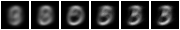
Now let us see how the event was chosen. Here are the slices and their underlying for each non-null derived variable state, \[ \{A_{\mathrm{b}} * \{\{(w,u)\}\}^{\mathrm{U}}~\%~\{w\} : (S,\cdot) \in Q * F^{\mathrm{T}},~(w,u) \in S,~u \neq \mathrm{null}\} \]
hrqb = hrfmul(uu2,ff,hrq)

ll = [(w,u) for (ss,_) in aall(hhaa(hrhh(uu2,hrhrred(hrqb,fder(ff))))) for (w,u) in ssll(ss) if u != ValStr("null")]

hrb1 = hrhrred(hrb,vvk|sset([w for (w,u) in ll]))

rpln([hhaa(hrhh(uu2,hrhrred(hrhrsel(hrb1,aahr(uu2,rr)),vars(rr)))) for (w,u) in ll for rr in [single(llss([(w,u)]),1)]])
# {({(<<<1,1>,n2>,1>, 0)}, 3927 % 1)}
# {({(<<<2,1>,n2>,1>, 0)}, 1534 % 1)}
# {({(<<<6,1>,n2>,1>, 0)}, 627 % 1)}
# {({(<<<16,1>,n2>,1>, 0)}, 230 % 1)}
# {({(<<<28,1>,n2>,1>, 0)}, 321 % 1)}
# {({(<<<52,1>,n2>,1>, 0)}, 175 % 1)}
# {({(<<<73,1>,n2>,1>, 0)}, 286 % 1)}
# {({(<<<103,1>,n2>,1>, 1)}, 52 % 1)}
# {({(<<<115,1>,n2>,1>, 0)}, 212 % 1)}

bmwrite(file,bmhstack([bmborder(1,hrbm(28,2,2,hrhrred(hrhrsel(hrb1,aahr(uu2,rr)),vvk))) for (w,u) in ll for rr in [single(llss([(w,u)]),1)]]))

bmwrite(file,bmhstack([bmborder(1,hrbm(28,2,2,qqhr(2,uu,vvk,fund(fdep(ff,sset([w])))))) for (w,u) in ll]))

Note that we are considering the reduced decomposition, $D_{\mathrm{r}}$, which can be indistinct, so the non-null derived variables do not necessarily correspond to just one path of the original decomposition, $D$. In this case they correspond to two paths,
# (0, [1, 2, 6, 28, 73, 115])
# ...
# (2, [1, 2, 6, 16, 52, 103])
# ...

bmwrite(file,bmhstack([bmborder(1,hrbm(28,1,2,hrhrred(hrs,vvk))) for (_,hrs) in pp[0]]))

bmwrite(file,bmhstack([bmborder(1,hrbm(28,1,2,hrhrred(hrs,vvk))) for (_,hrs) in pp[2]]))
Let us examine the level 1 nullable derived variables of the central region at (7;7),
def islevnull(x):
    if isinstance(x, VarPair):
        (w,c) = x._rep
        if isinstance(w, VarPair) and isinstance(c, VarStr) and c._rep == "(7;7)":
            (u,_) = w._rep
            if isinstance(u, VarPair):
                (_,g) = u._rep
                if isinstance(g, VarStr) and g._rep == "n":
                    return True
    return False

len([w for w in fvars(ff) if islevnull(w)])
16

ll = list(sset([(w,u) for (ss,_) in aall(hhaa(hrhh(uu2,hrhrred(hrqb,sset([w for w in fvars(ff) if islevnull(w)]))))) for (w,u) in ssll(ss) if u != ValStr("null")]))

hrb1 = hrhrred(hrb,vvk|sset([w for (w,u) in ll]))

rpln([hhaa(hrhh(uu2,hrhrred(hrhrsel(hrb1,aahr(uu2,rr)),vars(rr)))) for (w,u) in ll for rr in [single(llss([(w,u)]),1)]])
# {({(<<<<<1,1>,0>,n>,1>,(7;7)>, 0)}, 1784 % 1)}
# {({(<<<<<1,4>,0>,n>,1>,(7;7)>, 1)}, 1279 % 1)}

bmwrite(file,bmhstack([bmborder(1,hrbm(28,2,2,hrhrred(hrhrsel(hrb1,aahr(uu2,rr)),vvk))) for (w,u) in ll for rr in [single(llss([(w,u)]),1)]]))

bmmask = bminsert(bmempty(28*2,28*2),7*2-1,7*2-1,bmfull(15*2,15*2))

bmwrite(file,bmhstack([bmborder(1,bmmin(bmmask,0,0,hrbm(28,2,2,hrhrred(hrhrsel(hrb1,aahr(uu2,rr)),vvk)))) for (w,u) in ll for rr in [single(llss([(w,u)]),1)]]))

bmwrite(file,bmhstack([bmborder(1,hrbm(28,2,2,qqhr(2,uu,vvk,fund(fdep(ff,sset([w])))))) for (w,u) in ll]))

This frame detects the middle section of the five.
We can compare this region to the region, say, at (1;13),
def islevnull(x):
    if isinstance(x, VarPair):
        (w,c) = x._rep
        if isinstance(w, VarPair) and isinstance(c, VarStr) and c._rep == "(1;13)":
            (u,_) = w._rep
            if isinstance(u, VarPair):
                (_,g) = u._rep
                if isinstance(g, VarStr) and g._rep == "n":
                    return True
    return False

len([w for w in fvars(ff) if islevnull(w)])
9

ll = list(sset([(w,u) for (ss,_) in aall(hhaa(hrhh(uu2,hrhrred(hrqb,sset([w for w in fvars(ff) if islevnull(w)]))))) for (w,u) in ssll(ss) if u != ValStr("null")]))

hrb1 = hrhrred(hrb,vvk|sset([w for (w,u) in ll]))

rpln([hhaa(hrhh(uu2,hrhrred(hrhrsel(hrb1,aahr(uu2,rr)),vars(rr)))) for (w,u) in ll for rr in [single(llss([(w,u)]),1)]])
# {({(<<<<<1,1>,0>,n>,1>,(1;13)>, 1)}, 6458 % 1)}
# {({(<<<<<1,2>,0>,n>,1>,(1;13)>, 1)}, 1178 % 1)}

bmwrite(file,bmhstack([bmborder(1,hrbm(28,2,2,hrhrred(hrhrsel(hrb1,aahr(uu2,rr)),vvk))) for (w,u) in ll for rr in [single(llss([(w,u)]),1)]]))

bmmask = bminsert(bmempty(28*2,28*2),1*2-1,13*2-1,bmfull(15*2,15*2))

bmwrite(file,bmhstack([bmborder(1,bmmin(bmmask,0,0,hrbm(28,2,2,hrhrred(hrhrsel(hrb1,aahr(uu2,rr)),vvk)))) for (w,u) in ll for rr in [single(llss([(w,u)]),1)]]))

bmwrite(file,bmhstack([bmborder(1,hrbm(28,2,2,qqhr(2,uu,vvk,fund(fdep(ff,sset([w])))))) for (w,u) in ll]))

This frame detects the top right tip of the five.
We can compare again to the region at (4;7),
def islevnull(x):
    if isinstance(x, VarPair):
        (w,c) = x._rep
        if isinstance(w, VarPair) and isinstance(c, VarStr) and c._rep == "(4;7)":
            (u,_) = w._rep
            if isinstance(u, VarPair):
                (_,g) = u._rep
                if isinstance(g, VarStr) and g._rep == "n":
                    return True
    return False

len([w for w in fvars(ff) if islevnull(w)])
13

ll = list(sset([(w,u) for (ss,_) in aall(hhaa(hrhh(uu2,hrhrred(hrqb,sset([w for w in fvars(ff) if islevnull(w)]))))) for (w,u) in ssll(ss) if u != ValStr("null")]))

hrb1 = hrhrred(hrb,vvk|sset([w for (w,u) in ll]))

rpln([hhaa(hrhh(uu2,hrhrred(hrhrsel(hrb1,aahr(uu2,rr)),vars(rr)))) for (w,u) in ll for rr in [single(llss([(w,u)]),1)]])
# {({(<<<<<1,1>,0>,n>,1>,(4;7)>, 1)}, 5567 % 1)}
# {({(<<<<<1,2>,0>,n>,1>,(4;7)>, 1)}, 4233 % 1)}
# {({(<<<<<1,3>,0>,n>,1>,(4;7)>, 0)}, 1371 % 1)}

bmwrite(file,bmhstack([bmborder(1,hrbm(28,2,2,hrhrred(hrhrsel(hrb1,aahr(uu2,rr)),vvk))) for (w,u) in ll for rr in [single(llss([(w,u)]),1)]]))

bmmask = bminsert(bmempty(28*2,28*2),4*2-1,7*2-1,bmfull(15*2,15*2))

bmwrite(file,bmhstack([bmborder(1,bmmin(bmmask,0,0,hrbm(28,2,2,hrhrred(hrhrsel(hrb1,aahr(uu2,rr)),vvk)))) for (w,u) in ll for rr in [single(llss([(w,u)]),1)]]))

bmwrite(file,bmhstack([bmborder(1,hrbm(28,2,2,qqhr(2,uu,vvk,fund(fdep(ff,sset([w])))))) for (w,u) in ll]))

This frame detects the top arc of the five.
Now let us repeat the same analysis for the next event,
hrq = hrev([1],hrhrred(hr,vvk))

bmwrite(file,bmborder(1,hrbm(28,2,2,hrq)))
Now find the leaf slice of the query,
hrc = hrhrsel(hrb,hrhrred(hrfmul(uu2,ff,hrq),fder(ff)))

hrsize(hrc)
50

bmwrite(file,bmborder(1,hrbm(28,2,2,hrhrred(hrc,vvk))))

Here are the first 20 slice events,
hrc1 = hrhrred(hrc,vvk)

bmwrite(file,bmhstack([bmborder(1,hrbm(28,1,2,hrev([i],hrc1))) for i in range(min(20,hrsize(hrc1)))]))

The label variable is,
rpln(aall(hhaa(hrhh(uu1,hrhrred(hrc,vvl)))))
# ({(digit, 1)}, 49 % 1)
# ({(digit, 9)}, 1 % 1)
In this case the slice consists of nearly all ones.
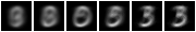
Here are the slices and their underlying for each non-null derived variable state,
hrqb = hrfmul(uu2,ff,hrq)

ll = [(w,u) for (ss,_) in aall(hhaa(hrhh(uu2,hrhrred(hrqb,fder(ff))))) for (w,u) in ssll(ss) if u != ValStr("null")]

hrb1 = hrhrred(hrb,vvk|sset([w for (w,u) in ll]))

rpln([hhaa(hrhh(uu2,hrhrred(hrhrsel(hrb1,aahr(uu2,rr)),vars(rr)))) for (w,u) in ll for rr in [single(llss([(w,u)]),1)]])
# {({(<<<1,1>,n2>,1>, 1)}, 3573 % 1)}
# {({(<<<3,1>,n2>,1>, 1)}, 1653 % 1)}
# {({(<<<10,1>,n2>,1>, 1)}, 540 % 1)}
# {({(<<<14,1>,n2>,1>, 0)}, 1469 % 1)}
# {({(<<<24,1>,n2>,1>, 0)}, 280 % 1)}
# {({(<<<32,1>,n2>,1>, 1)}, 670 % 1)}
# {({(<<<66,1>,n2>,1>, 1)}, 106 % 1)}
# {({(<<<88,1>,n2>,1>, 0)}, 1314 % 1)}
# {({(<<<107,1>,n2>,1>, 1)}, 484 % 1)}
# {({(<<<124,1>,n2>,1>, 1)}, 250 % 1)}

bmwrite(file,bmhstack([bmborder(1,hrbm(28,2,2,hrhrred(hrhrsel(hrb1,aahr(uu2,rr)),vvk))) for (w,u) in ll for rr in [single(llss([(w,u)]),1)]]))

bmwrite(file,bmhstack([bmborder(1,hrbm(28,2,2,qqhr(2,uu,vvk,fund(fdep(ff,sset([w])))))) for (w,u) in ll]))

Two level over centred square regions of 11x11 pixels
Let us consider a two level model which consists of 5x5 frames of Centred square regions of 11x11 pixels - see Model induction. The model NIST_model26.json is induced by NIST_engine26.py.
We shall analyse it with the 7,500 events subset of the sample,
from NISTDev import *

(uu,hrtr) = nistTrainBucketedIO(2)

digit = VarStr("digit")
vv = uvars(uu)
vvl = sset([digit])
vvk = vv - vvl

hr = hrev([i for i in range(hrsize(hrtr)) if i % 8 == 0],hrtr)

hrsize(hr)
7500

df = dfIO('./NIST_model26.json')

uu1 = uunion(uu,fsys(dfff(df)))

len(dfund(df))
427

len(fvars(dfff(df)))
5671

(wmax,lmax,xmax,omax,bmax,mmax,umax,pmax,fmax,mult,seed) = (2**11, 8, 2**10, 30, (30*3), 3, 2**8, 1, 127, 1, 5)

summation(mult,seed,uu1,df,hr)
# (206488.07062685423, 98883.55460646778)
We can compare this to the all pixels 1-level model, (132688.71288792725, 64806.344175194274). The 2-level model is more highly aligned, similar to the other 2-level models, Two level over 10x10 regions, (190022.26132400509, 89892.41155833867), and Two level over 15x15 regions, (174749.41491485896, 78155.5550910946).
Below is an image of the fud decomposition, and adjacent is an image of the fud underlying superimposed on the slices,

A magnified image of the fud underlying superimposed on the averaged slice, can be seen at Model 26.
We can see that the fud underlying clusters are larger in general than for the 1-level model. The paths vary in length from three fuds to 17 fuds. The tree is a little more uniform than the 1-level model, reflected in the higher alignment. The tree is less uniform than for the other 2-level models, Two level over 10x10 regions and Two level over 15x15 regions.
Let us reduce the decomposition to make it more managable,
dfr = dfred(uu1,df,hr)

len(dfund(dfr))
412

len(fder(dfff(dfr)))
127

len(fvars(dfff(dfr)))
2834
Let us examine the slices, $P = \mathrm{paths}(A * D_{\mathrm{r}})$,
def variablesVariableFud(x):
    if isinstance(x, VarPair):
        (w,_) = x._rep
        if isinstance(w, VarPair):
            (u,_) = w._rep
            if isinstance(u, VarPair):
                (f,_) = u._rep
            return f
    return VarInt(0)

def fid(ff):
    return variablesVariableFud(fder(ff)[0])

pp = treesPaths(hrmult(uu1,dfr,hr))

rpln([(i,[fid(ff) for ((_,ff),_) in ll]) for (i,ll) in enumerate(pp)])
# (0, [1, 2, 3, 5, 7, 8, 10, 15, 19, 23, 35, 48, 58, 70, 85, 100, 123])
# (1, [1, 2, 3, 5, 7, 8, 10, 15, 19, 23, 126])
# (2, [1, 2, 3, 5, 7, 8, 10, 15, 19, 94])
# ...
# (34, [1, 4, 11, 17, 22, 30, 86, 116])
# (35, [1, 4, 11, 17, 22, 30, 120])
# (36, [1, 4, 11, 17, 22, 107])
# (37, [1, 4, 11, 17, 56, 99, 124])
# (38, [1, 4, 11, 49, 64, 127])

rpln([(i,[hrsize(hr) for (_,hr) in ll]) for (i,ll) in enumerate(pp)])
# (0, [7500, 4983, 3517, 2373, 1648, 1346, 1091, 858, 649, 543, 361, 282, 264, 211, 176, 155, 129])
# (1, [7500, 4983, 3517, 2373, 1648, 1346, 1091, 858, 649, 543, 182])
# (2, [7500, 4983, 3517, 2373, 1648, 1346, 1091, 858, 649, 106])
# ...
# (34, [7500, 2517, 913, 663, 403, 318, 280, 220])
# (35, [7500, 2517, 913, 663, 403, 318, 280])
# (36, [7500, 2517, 913, 663, 403, 85])
# (37, [7500, 2517, 913, 663, 260, 179, 131])
# (38, [7500, 2517, 913, 250, 197, 114])
Imaging the reduced decomposition slices,
file = "NIST.bmp"

bmwrite(file,ppbm2(uu,vvk,28,1,2,pp))

bmwrite(file,ppbm(uu,vvk,28,1,2,pp))
Again, the reduced decomposition is similar to the original decomposition.
The underlying tuple of the root slice is $\mathrm{und}(F)$, where $((\cdot,F),\cdot) = P_{1,1}$,
((_,ff),hrs) = pp[0][0]

len(fund(ff))
42

bmwrite(file,bmborder(1,bmmax(hrbm(28,3,2,hrhrred(hrs,vvk)),0,0,hrbm(28,3,2,qqhr(2,uu,vvk,fund(ff))))))

We can see that the root slice depends on an underlying cluster that is larger than the corresponding cluster for the root slice in the 1-level model. It is also in a different location.
The first child slice of the second column has size 4983,
((_,ff),hrs) = pp[0][1]

len(fund(ff))
42

bmwrite(file,bmborder(1,bmmax(hrbm(28,3,2,hrhrred(hrs,vvk)),0,0,hrbm(28,3,2,qqhr(2,uu,vvk,fund(ff))))))

Again, we can see that the root slice depends on a larger cluster of the substrate than in the 1-level model.
Now let us query the model with a sample event to see how it is being classified. First, consider the fud decomposition fud, $F = D_{\mathrm{r}}^{\mathrm{F}}$,
ff = dfnul(uu1,dfr,2)

len(fvars(ff))
3211

len(fder(ff))
127

list(fder(ff))[:5]
# [<<<1,1>,n2>,1>, <<<2,1>,n2>,1>, <<<3,1>,n2>,1>, <<<4,1>,n2>,1>, <<<5,1>,n2>,1>]
Now apply the model to the sample history, $A_{\mathrm{b}} = A * \prod \mathrm{his}(F)$,
uu2 = uunion(uu,fsys(ff))

hrb = hrfmul(uu2,ff,hr)

hrsize(hrb)
7500

len(hrvars(hrb))
3584
Choose, for example, the first event $Q = \{S\}^{\mathrm{U}}$, where $S \in (A\%V_{\mathrm{k}})^{\mathrm{S}}$,
hrq = hrev([0],hrhrred(hr,vvk))

bmwrite(file,bmborder(1,hrbm(28,2,2,hrq)))
Now find the leaf slice of the query, $A_{\mathrm{c}} = A_{\mathrm{b}} * (Q * F^{\mathrm{T}})$,
hrc = hrhrsel(hrb,hrhrred(hrfmul(uu2,ff,hrq),fder(ff)))

hrsize(hrc)
47

bmwrite(file,bmborder(1,hrbm(28,2,2,hrhrred(hrc,vvk))))

Here are the first 20 slice events, $A_{\mathrm{c}}~\%~V_{\mathrm{k}}$,
hrc1 = hrhrred(hrc,vvk)

bmwrite(file,bmhstack([bmborder(1,hrbm(28,1,2,hrev([i],hrc1))) for i in range(min(20,hrsize(hrc1)))]))

The label variable is, $A_{\mathrm{c}}~\%~V_{\mathrm{l}}$,
rpln(aall(hhaa(hrhh(uu1,hrhrred(hrc,vvl)))))
# ({(digit, 2)}, 4 % 1)
# ({(digit, 3)}, 27 % 1)
# ({(digit, 4)}, 1 % 1)
# ({(digit, 5)}, 7 % 1)
# ({(digit, 7)}, 2 % 1)
# ({(digit, 8)}, 1 % 1)
# ({(digit, 9)}, 5 % 1)
The modal label is three, but there are some fives.
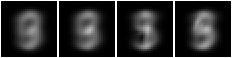
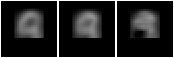
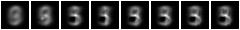
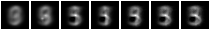
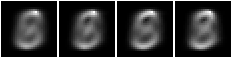
Now let us see how the event was chosen. Here are the slices and their underlying for each non-null derived variable state, \[ \{A_{\mathrm{b}} * \{\{(w,u)\}\}^{\mathrm{U}}~\%~\{w\} : (S,\cdot) \in Q * F^{\mathrm{T}},~(w,u) \in S,~u \neq \mathrm{null}\} \]
hrqb = hrfmul(uu2,ff,hrq)

ll = [(w,u) for (ss,_) in aall(hhaa(hrhh(uu2,hrhrred(hrqb,fder(ff))))) for (w,u) in ssll(ss) if u != ValStr("null")]

hrb1 = hrhrred(hrb,vvk|sset([w for (w,u) in ll]))

rpln([hhaa(hrhh(uu2,hrhrred(hrhrsel(hrb1,aahr(uu2,rr)),vars(rr)))) for (w,u) in ll for rr in [single(llss([(w,u)]),1)]])
# {({(<<<1,1>,n2>,1>, 1)}, 2517 % 1)}
# {({(<<<4,1>,n2>,1>, 1)}, 913 % 1)}
# {({(<<<11,1>,n2>,1>, 0)}, 663 % 1)}
# {({(<<<17,1>,n2>,1>, 0)}, 403 % 1)}
# {({(<<<22,1>,n2>,1>, 0)}, 318 % 1)}
# {({(<<<30,1>,n2>,1>, 0)}, 280 % 1)}
# {({(<<<86,1>,n2>,1>, 1)}, 60 % 1)}
# {({(<<<120,1>,n2>,1>, 0)}, 207 % 1)}

bmwrite(file,bmhstack([bmborder(1,hrbm(28,2,2,hrhrred(hrhrsel(hrb1,aahr(uu2,rr)),vvk))) for (w,u) in ll for rr in [single(llss([(w,u)]),1)]]))

bmwrite(file,bmhstack([bmborder(1,hrbm(28,2,2,qqhr(2,uu,vvk,fund(fdep(ff,sset([w])))))) for (w,u) in ll]))

Note that we are considering the reduced decomposition, $D_{\mathrm{r}}$, which can be indistinct, so the non-null derived variables do not necessarily correspond to just one path of the original decomposition, $D$. In this case they correspond to two paths,
# ...
# (34, [1, 4, 11, 17, 22, 30, 86, 116])
# (35, [1, 4, 11, 17, 22, 30, 120])
# ...

bmwrite(file,bmhstack([bmborder(1,hrbm(28,1,2,hrhrred(hrs,vvk))) for (_,hrs) in pp[34]]))

bmwrite(file,bmhstack([bmborder(1,hrbm(28,1,2,hrhrred(hrs,vvk))) for (_,hrs) in pp[35]]))
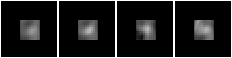
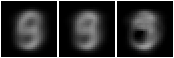
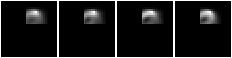
Let us examine the level 1 nullable derived variables of the central region at (10;10),
def islevnull(x):
    if isinstance(x, VarPair):
        (w,c) = x._rep
        if isinstance(w, VarPair) and isinstance(c, VarStr) and c._rep == "(10;10)":
            (u,_) = w._rep
            if isinstance(u, VarPair):
                (_,g) = u._rep
                if isinstance(g, VarStr) and g._rep == "n":
                    return True
    return False

len([w for w in fvars(ff) if islevnull(w)])
25

ll = list(sset([(w,u) for (ss,_) in aall(hhaa(hrhh(uu2,hrhrred(hrqb,sset([w for w in fvars(ff) if islevnull(w)]))))) for (w,u) in ssll(ss) if u != ValStr("null")]))

hrb1 = hrhrred(hrb,vvk|sset([w for (w,u) in ll]))

rpln([hhaa(hrhh(uu2,hrhrred(hrhrsel(hrb1,aahr(uu2,rr)),vars(rr)))) for (w,u) in ll for rr in [single(llss([(w,u)]),1)]])
# {({(<<<<<1,0>,0>,n>,1>,(10;10)>, 1)}, 3763 % 1)}
# {({(<<<<<1,1>,0>,n>,1>,(10;10)>, 0)}, 1539 % 1)}
# {({(<<<<<1,3>,0>,n>,1>,(10;10)>, 0)}, 913 % 1)}
# {({(<<<<<1,5>,0>,n>,1>,(10;10)>, 1)}, 743 % 1)}
# {({(<<<<<1,9>,0>,n>,1>,(10;10)>, 1)}, 492 % 1)}
# {({(<<<<<1,19>,0>,n>,1>,(10;10)>, 1)}, 357 % 1)}
# {({(<<<<<1,34>,0>,n>,1>,(10;10)>, 1)}, 200 % 1)}

bmwrite(file,bmhstack([bmborder(1,hrbm(28,2,2,hrhrred(hrhrsel(hrb1,aahr(uu2,rr)),vvk))) for (w,u) in ll for rr in [single(llss([(w,u)]),1)]]))

bmmask = bminsert(bmempty(28*2,28*2),10*2-1,10*2-1,bmfull(11*2,11*2))

bmwrite(file,bmhstack([bmborder(1,bmmin(bmmask,0,0,hrbm(28,2,2,hrhrred(hrhrsel(hrb1,aahr(uu2,rr)),vvk)))) for (w,u) in ll for rr in [single(llss([(w,u)]),1)]]))

bmwrite(file,bmhstack([bmborder(1,hrbm(28,2,2,qqhr(2,uu,vvk,fund(fdep(ff,sset([w])))))) for (w,u) in ll]))

This frame detects the middle section of the five.
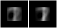
We can compare this region to the region, say, at (1;13),
def islevnull(x):
    if isinstance(x, VarPair):
        (w,c) = x._rep
        if isinstance(w, VarPair) and isinstance(c, VarStr) and c._rep == "(1;13)":
            (u,_) = w._rep
            if isinstance(u, VarPair):
                (_,g) = u._rep
                if isinstance(g, VarStr) and g._rep == "n":
                    return True
    return False

len([w for w in fvars(ff) if islevnull(w)])
15

ll = list(sset([(w,u) for (ss,_) in aall(hhaa(hrhh(uu2,hrhrred(hrqb,sset([w for w in fvars(ff) if islevnull(w)]))))) for (w,u) in ssll(ss) if u != ValStr("null")]))

hrb1 = hrhrred(hrb,vvk|sset([w for (w,u) in ll]))

rpln([hhaa(hrhh(uu2,hrhrred(hrhrsel(hrb1,aahr(uu2,rr)),vars(rr)))) for (w,u) in ll for rr in [single(llss([(w,u)]),1)]])
# {({(<<<<<1,0>,0>,n>,1>,(1;13)>, 1)}, 2151 % 1)}
# {({(<<<<<1,1>,0>,n>,1>,(1;13)>, 1)}, 1393 % 1)}
# {({(<<<<<1,2>,0>,n>,1>,(1;13)>, 1)}, 1145 % 1)}
# {({(<<<<<1,4>,0>,n>,1>,(1;13)>, 1)}, 748 % 1)}

bmwrite(file,bmhstack([bmborder(1,hrbm(28,2,2,hrhrred(hrhrsel(hrb1,aahr(uu2,rr)),vvk))) for (w,u) in ll for rr in [single(llss([(w,u)]),1)]]))

bmmask = bminsert(bmempty(28*2,28*2),1*2-1,13*2-1,bmfull(11*2,11*2))

bmwrite(file,bmhstack([bmborder(1,bmmin(bmmask,0,0,hrbm(28,2,2,hrhrred(hrhrsel(hrb1,aahr(uu2,rr)),vvk)))) for (w,u) in ll for rr in [single(llss([(w,u)]),1)]]))

bmwrite(file,bmhstack([bmborder(1,hrbm(28,2,2,qqhr(2,uu,vvk,fund(fdep(ff,sset([w])))))) for (w,u) in ll]))

This frame detects the top right tip of the five.
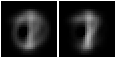
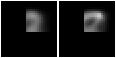
We can compare again to the region at (7;10),
def islevnull(x):
    if isinstance(x, VarPair):
        (w,c) = x._rep
        if isinstance(w, VarPair) and isinstance(c, VarStr) and c._rep == "(7;10)":
            (u,_) = w._rep
            if isinstance(u, VarPair):
                (_,g) = u._rep
                if isinstance(g, VarStr) and g._rep == "n":
                    return True
    return False

len([w for w in fvars(ff) if islevnull(w)])
16

ll = list(sset([(w,u) for (ss,_) in aall(hhaa(hrhh(uu2,hrhrred(hrqb,sset([w for w in fvars(ff) if islevnull(w)]))))) for (w,u) in ssll(ss) if u != ValStr("null")]))

hrb1 = hrhrred(hrb,vvk|sset([w for (w,u) in ll]))

rpln([hhaa(hrhh(uu2,hrhrred(hrhrsel(hrb1,aahr(uu2,rr)),vars(rr)))) for (w,u) in ll for rr in [single(llss([(w,u)]),1)]])
# {({(<<<<<1,0>,0>,n>,1>,(7;10)>, 0)}, 5249 % 1)}

bmwrite(file,bmhstack([bmborder(1,hrbm(28,2,2,hrhrred(hrhrsel(hrb1,aahr(uu2,rr)),vvk))) for (w,u) in ll for rr in [single(llss([(w,u)]),1)]]))

bmmask = bminsert(bmempty(28*2,28*2),7*2-1,10*2-1,bmfull(11*2,11*2))

bmwrite(file,bmhstack([bmborder(1,bmmin(bmmask,0,0,hrbm(28,2,2,hrhrred(hrhrsel(hrb1,aahr(uu2,rr)),vvk)))) for (w,u) in ll for rr in [single(llss([(w,u)]),1)]]))

bmwrite(file,bmhstack([bmborder(1,hrbm(28,2,2,qqhr(2,uu,vvk,fund(fdep(ff,sset([w])))))) for (w,u) in ll]))


This frame detects the top arc of the five. In this case the central pixel is not set.
Now let us repeat the same analysis for the next event,
hrq = hrev([1],hrhrred(hr,vvk))

bmwrite(file,bmborder(1,hrbm(28,2,2,hrq)))
Now find the leaf slice of the query,
hrc = hrhrsel(hrb,hrhrred(hrfmul(uu2,ff,hrq),fder(ff)))

hrsize(hrc)
81

bmwrite(file,bmborder(1,hrbm(28,2,2,hrhrred(hrc,vvk))))

Here are the first 20 slice events,
hrc1 = hrhrred(hrc,vvk)

bmwrite(file,bmhstack([bmborder(1,hrbm(28,1,2,hrev([i],hrc1))) for i in range(min(20,hrsize(hrc1)))]))

The label variable is,
rpln(aall(hhaa(hrhh(uu1,hrhrred(hrc,vvl)))))
# ({(digit, 1)}, 73 % 1)
# ({(digit, 4)}, 1 % 1)
# ({(digit, 7)}, 6 % 1)
# ({(digit, 9)}, 1 % 1)
In this case the slice consists mostly of ones.
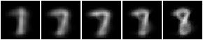
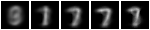
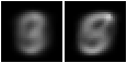
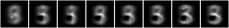
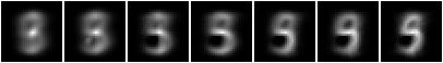
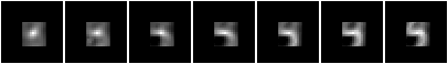
Here are the slices and their underlying for each non-null derived variable state,
hrqb = hrfmul(uu2,ff,hrq)

ll = [(w,u) for (ss,_) in aall(hhaa(hrhh(uu2,hrhrred(hrqb,fder(ff))))) for (w,u) in ssll(ss) if u != ValStr("null")]

hrb1 = hrhrred(hrb,vvk|sset([w for (w,u) in ll]))

rpln([hhaa(hrhh(uu2,hrhrred(hrhrsel(hrb1,aahr(uu2,rr)),vars(rr)))) for (w,u) in ll for rr in [single(llss([(w,u)]),1)]])
# {({(<<<1,1>,n2>,1>, 1)}, 2517 % 1)}
# {({(<<<4,1>,n2>,1>, 1)}, 913 % 1)}
# {({(<<<11,1>,n2>,1>, 0)}, 663 % 1)}
# {({(<<<17,1>,n2>,1>, 1)}, 260 % 1)}
# {({(<<<56,1>,n2>,1>, 1)}, 81 % 1)}

bmwrite(file,bmhstack([bmborder(1,hrbm(28,2,2,hrhrred(hrhrsel(hrb1,aahr(uu2,rr)),vvk))) for (w,u) in ll for rr in [single(llss([(w,u)]),1)]]))

bmwrite(file,bmhstack([bmborder(1,hrbm(28,2,2,qqhr(2,uu,vvk,fund(fdep(ff,sset([w])))))) for (w,u) in ll]))