Predicting digit without modelling
MNIST - handwritten digits/Predicting digit without modelling
Sections
Introduction
The sample query variables predict digit. That is, there is a functional or causal relationship between the query variables and the label variables, $(A\%V_{\mathrm{k}})^{\mathrm{FS}} \to (A\%V_{\mathrm{l}})^{\mathrm{FS}}$. So the label entropy or query conditional entropy is zero. See Entropy and alignment. The label entropy is \[ \begin{eqnarray} \mathrm{lent}(A,W,L)~:=~\mathrm{entropy}(A~\%~(W \cup L)) - \mathrm{entropy}(A~\%~W) \end{eqnarray} \]
First load the training sample,
from NISTDev import *

(uu,hrtr) = nistTrainBucketedIO(2)

digit = VarStr("digit")
vv = uvars(uu)
vvl = sset([digit])
vvk = vv - vvl

hr = hrev([i for i in range(hrsize(hrtr)) if i % 8 == 0],hrtr)
The shuffle is $A_{\mathrm{r}}$,
hrr = historyRepasShuffle_u(hr,1)
Then $\mathrm{lent}(A,V_{\mathrm{k}},V_{\mathrm{l}}) = 0$,
hrlent(uu,hr,vvk,vvl)
0.0
Note that we have redefined hrlent in module NISTDev to improve the performance.
1-tuple
We can determine which of the query variables has the least conditional entropy, \[ \begin{eqnarray} \{(\mathrm{lent}(A,\{w\},V_{\mathrm{l}}),~w) : w \in V_{\mathrm{k}}\} \end{eqnarray} \]
ll = list(sset([(hrlent(uu,hr,sset([w]),vvl),w) for w in vvk]))

rpln(ll[:20])
# (2.106715914339201, <13,15>)
# (2.1123060297815157, <14,15>)
# (2.1332577705312126, <15,15>)
# (2.134076004038435, <22,10>)
# (2.136893962468214, <20,11>)
# (2.1372105576567395, <21,10>)
# (2.14168787689367, <20,12>)
# (2.1419488804233735, <21,11>)
# (2.1420641036112578, <12,15>)
# (2.143524082463724, <22,11>)
# (2.1438457401658626, <16,15>)
# (2.1453000849733357, <23,11>)
# (2.146147540554603, <14,14>)
# (2.148859975095617, <21,9>)
# (2.149828008927548, <24,13>)
# (2.1506649095818275, <21,12>)
# (2.1514776557663415, <17,15>)
# (2.1536449181562007, <15,18>)
# (2.1554691036826017, <23,12>)
# (2.155476320456197, <20,10>)
The top pixel is <13,15>. Here it is overlaid on the average, $\hat{A}\%V_{\mathrm{k}}$,
file = "NIST.bmp"

hrbmav = hrbm(28,3,2,hrhrred(hr,vvk))

bmwrite(file,bmborder(1,bmmax(hrbmav,0,0,hrbm(28,3,2,qqhr(2,uu,vvk,sset([ll[0][1]]))))))

Imaging the 2 states ordered by size descending, $A~\%~\{\mathrm{<13,15>}\}$,
v1315 = stringsVariable("<13,15>")

pp = list(reversed(list(sset([(b,a) for (a,b) in aall(araa(uu,hrred(hr,sset([v1315]))))]))))[:20]

[int(a) for (a,b) in pp]
# [4765, 2735]

bmwrite(file,bmhstack([bmborder(1,hrbm(28,3,2,hrhrred(hrhrsel(hr,aahr(uu,single(ss,1))),vvk))) for (_,ss) in pp]))
The top 20 are $\mathrm{topd}(20)(L)$, where $L = \{(w,~\mathrm{lent}(A,\{w\},V_{\mathrm{l}})) : w \in V_{\mathrm{k}}\}$,
bmwrite(file,bmborder(1,bmmax(hrbmav,0,0,hrbm(28,3,2,qqhr(2,uu,vvk,sset([v for (_,v) in ll[:20]]))))))

The top 100 are $\mathrm{topd}(100)(L)$,
bmwrite(file,bmborder(1,bmmax(hrbmav,0,0,hrbm(28,3,2,qqhr(2,uu,vvk,sset([v for (_,v) in ll[:100]]))))))

The bottom 20 pixels are $\mathrm{botd}(20)(L)$,
rpln(ll[-20:])
# (2.3018362154122483, <27,5>)
# (2.3018362154122483, <27,23>)
# (2.3018362154122483, <27,24>)
# (2.3018362154122483, <27,25>)
# (2.3018362154122483, <27,26>)
# (2.3018362154122483, <27,27>)
# (2.3018362154122483, <27,28>)
# (2.3018362154122483, <28,1>)
# (2.3018362154122483, <28,2>)
# (2.3018362154122483, <28,3>)
# (2.3018362154122483, <28,4>)
# (2.3018362154122483, <28,5>)
# (2.3018362154122483, <28,6>)
# (2.3018362154122483, <28,7>)
# (2.3018362154122483, <28,23>)
# (2.3018362154122483, <28,24>)
# (2.3018362154122483, <28,25>)
# (2.3018362154122483, <28,26>)
# (2.3018362154122483, <28,27>)
# (2.3018362154122483, <28,28>)
This may be compared to the entropy of the label variables, $\mathrm{entropy}(A\%V_{\mathrm{l}})$,
ent(araa(uu,hrred(hr,vvl)))
2.3018362154122483

bmwrite(file,bmborder(1,bmmax(hrbmav,0,0,hrbm(28,3,2,qqhr(2,uu,vvk,sset([v for (e,v) in ll if e >= 2.3018362154122483]))))))

Pixel <13,15> has the least conditional entropy, and so is more predictive of digit, $\mathrm{lent}(A,\{\mathrm{<13,15>}\},V_{\mathrm{l}})$,
hrlent(uu,hr,sset([v1315]),vvl)
2.106715914339201
The reduction is $A~\%~\{\mathrm{<13,15>}\}$,
rpln(aall(araa(uu,hrred(hr,sset([v1315])|vvl))))
# ({(digit, 0), (<13,15>, 0)}, 704 % 1)
# ({(digit, 0), (<13,15>, 1)}, 39 % 1)
# ({(digit, 1), (<13,15>, 0)}, 58 % 1)
# ({(digit, 1), (<13,15>, 1)}, 764 % 1)
# ({(digit, 2), (<13,15>, 0)}, 568 % 1)
# ({(digit, 2), (<13,15>, 1)}, 170 % 1)
# ({(digit, 3), (<13,15>, 0)}, 168 % 1)
# ({(digit, 3), (<13,15>, 1)}, 577 % 1)
# ({(digit, 4), (<13,15>, 0)}, 670 % 1)
# ({(digit, 4), (<13,15>, 1)}, 76 % 1)
# ({(digit, 5), (<13,15>, 0)}, 442 % 1)
# ({(digit, 5), (<13,15>, 1)}, 278 % 1)
# ({(digit, 6), (<13,15>, 0)}, 534 % 1)
# ({(digit, 6), (<13,15>, 1)}, 173 % 1)
# ({(digit, 7), (<13,15>, 0)}, 692 % 1)
# ({(digit, 7), (<13,15>, 1)}, 75 % 1)
# ({(digit, 8), (<13,15>, 0)}, 349 % 1)
# ({(digit, 8), (<13,15>, 1)}, 405 % 1)
# ({(digit, 9), (<13,15>, 0)}, 580 % 1)
# ({(digit, 9), (<13,15>, 1)}, 178 % 1)
We can determine minimum subsets of the query variables that are causal or predictive by using the conditional entropy tuple set builder. We shall calculate the shuffle content derived alignment and the size-volume-sized-shuffle relative entropy. \[ \{(\mathrm{lent}(A,M,V_{\mathrm{l}}),~M) : M \in \mathrm{botd}(\mathrm{qmax})(\mathrm{elements}(Z_{P,A,\mathrm{L}}))\} \] First load the test sample and select a subset of 1000 events $A_{\mathrm{te}}$,
(_,hrte) = nistTestBucketedIO(2)

hrsize(hrte)
10000

hrq = hrev([i for i in range(hrsize(hrte)) if i % 10 == 0],hrte)

hrsize(hrq)
1000
Now we do the conditional entropy minimise,
def buildcondrr(vvl,aa,kmax,omax,qmax):
    return sset([(b,a) for (a,b) in parametersBuilderConditionalVarsRepa(kmax,omax,qmax,vvl,aa).items()])
(kmax,omax,qmax) = (1, 60, 10)

ll = buildcondrr(vvl,hr,kmax,omax,qmax)

rpln(ll)
# (2.106715914339201, {<13,15>})
# (2.1123060297815157, {<14,15>})
# (2.1332577705312126, {<15,15>})
# (2.134076004038435, {<22,10>})
# (2.136893962468214, {<20,11>})
# (2.1372105576567395, {<21,10>})
# (2.14168787689367, {<20,12>})
# (2.1419488804233735, {<21,11>})
# (2.1420641036112578, {<12,15>})
# (2.143524082463724, {<22,11>})
Let us sort by shuffle content derived alignment descending. Let $L = \mathrm{botd}(\mathrm{qmax})(\mathrm{elements}(Z_{P,A,\mathrm{L}}))$. Then calculate \[ \{(\mathrm{algn}(A\%X)-\mathrm{algn}(A_{\mathrm{r}}\%X),~X) : (e,X) \in L\} \]
rpln(reversed(list(sset([(algn(aa1)-algn(aar1),xx) for (e,xx) in ll for aa1 in [hhaa(hrhh(uu,hrhrred(hr,xx)))] for aar1 in [hhaa(hrhh(uu,hrhrred(hrr,xx)))]]))))
# (0.0, {<22,11>})
# (0.0, {<22,10>})
# (0.0, {<21,11>})
# (0.0, {<21,10>})
# (0.0, {<20,12>})
# (0.0, {<20,11>})
# (0.0, {<15,15>})
# (0.0, {<14,15>})
# (0.0, {<13,15>})
# (0.0, {<12,15>})
and by size-volume-sized-shuffle relative entropy descending, \[ \{(\mathrm{rent}(A~\%~X,~Z_X * \hat{A}_{\mathrm{r}}~\%~X),~X) : (e,X) \in L\} \] where $Z_X = \mathrm{scalar}(|X^{\mathrm{C}}|)$,
def vsize(uu,xx,aa):
    return resize(vol(uu,xx),aa)

rpln(reversed(list(sset([(rent(aa1,vaar1),xx) for (e,xx) in ll for aa1 in [hhaa(hrhh(uu,hrhrred(hr,xx)))] for vaar1 in [vsize(uu,xx,hhaa(hrhh(uu,hrhrred(hrr,xx))))]]))))
# (2.7622348852673895e-13, {<12,15>})
# (2.737809978725636e-13, {<14,15>})
# (2.2959412149248237e-13, {<15,15>})
# (-4.884981308350689e-15, {<13,15>})
# (-6.439293542825908e-14, {<20,12>})
# (-1.6564527527407336e-13, {<22,11>})
# (-2.0516921495072893e-13, {<22,10>})
# (-3.157474282033945e-13, {<20,11>})
# (-4.89386309254769e-13, {<21,10>})
# (-6.794564910705958e-13, {<21,11>})
Choose the top tuple $X$,
xx = sset(map(stringsVariable,["<13,15>"]))

len(xx)
1
The label entropy, $\mathrm{lent}(A,X,V_{\mathrm{l}})$, is,
hrlent(uu,hr,xx,vvl)
2.106715914339201
This tuple has a volume of $|X^{\mathrm{C}}| = 2$,
vol(uu,xx)
2
Now consider the query effectiveness against the test set, $\mathrm{size}(A_{\mathrm{te}} * (A\%X)^{\mathrm{F}})$,
size(mul(hhaa(hrhh(uu,hrhrred(hrq,xx))),eff(hhaa(hrhh(uu,hrhrred(hr,xx))))))
# 1000 % 1
So there exists a prediction for each of the test set for the mono-variate tuple.
2-tuple
(kmax,omax,qmax) = (2, 10, 10)

ll = buildcondrr(vvl,hr,kmax,omax,qmax)

rpln(ll)
# (1.9278815272185972, {<14,15>, <17,15>})
# (1.9308806609242304, {<13,15>, <16,15>})
# (1.9312459077976916, {<13,15>, <17,15>})
# (1.9345734579988292, {<13,15>, <22,10>})
# (1.9378630043953957, {<13,15>, <20,11>})
# (1.9389377983376284, {<13,15>, <21,10>})
# (1.9411899963428647, {<14,15>, <22,10>})
# (1.9421337966096712, {<13,15>, <21,11>})
# (1.9422336675359633, {<14,15>, <20,11>})
# (1.9431673552302653, {<13,15>, <22,11>})

rpln(reversed(list(sset([(algn(aa1)-algn(aar1),xx) for (e,xx) in ll for aa1 in [hhaa(hrhh(uu,hrhrred(hr,xx)))] for aar1 in [hhaa(hrhh(uu,hrhrred(hrr,xx)))]]))))
# (41.79031505694729, {<13,15>, <16,15>})
# (6.347144837862288, {<13,15>, <21,10>})
# (5.72152054469916, {<13,15>, <20,11>})
# (3.883178704774764, {<14,15>, <17,15>})
# (1.7061474604197429, {<14,15>, <22,10>})
# (1.269607648246165, {<13,15>, <22,10>})
# (0.2197908734815428, {<13,15>, <22,11>})
# (-0.16175869062863057, {<14,15>, <20,11>})
# (-1.2173589845770039, {<13,15>, <21,11>})
# (-1.665466231672326, {<13,15>, <17,15>})

rpln(reversed(list(sset([(rent(aa1,vaar1),xx) for (e,xx) in ll for aa1 in [hhaa(hrhh(uu,hrhrred(hr,xx)))] for vaar1 in [vsize(uu,xx,hhaa(hrhh(uu,hrhrred(hrr,xx))))]]))))
# (0.03396160918549729, {<13,15>, <16,15>})
# (0.007169898198625901, {<13,15>, <21,10>})
# (0.002702072763310248, {<13,15>, <20,11>})
# (0.0013297760191726127, {<14,15>, <17,15>})
# (0.001091885316609087, {<14,15>, <22,10>})
# (0.0007863858921490774, {<13,15>, <22,10>})
# (0.0007540216018115942, {<13,15>, <17,15>})
# (0.00012768804279961188, {<13,15>, <21,11>})
# (5.584813210646189e-05, {<13,15>, <22,11>})
# (2.660226409112454e-05, {<14,15>, <20,11>})

xx = sset(map(stringsVariable,["<13,15>","<16,15>"]))

len(xx)
2

hrlent(uu,hr,xx,vvl)
1.9308806609242304

vol(uu,xx)
4

size(mul(hhaa(hrhh(uu,hrhrred(hrq,xx))),eff(hhaa(hrhh(uu,hrhrred(hr,xx))))))
# 1000 % 1

rpln(aall(araa(uu,hrred(hr,xx|vvl))))
# ({(digit, 0), (<13,15>, 0), (<16,15>, 0)}, 699 % 1)
# ({(digit, 0), (<13,15>, 0), (<16,15>, 1)}, 5 % 1)
# ({(digit, 0), (<13,15>, 1), (<16,15>, 0)}, 33 % 1)
# ({(digit, 0), (<13,15>, 1), (<16,15>, 1)}, 6 % 1)
# ({(digit, 1), (<13,15>, 0), (<16,15>, 0)}, 19 % 1)
# ({(digit, 1), (<13,15>, 0), (<16,15>, 1)}, 39 % 1)
# ({(digit, 1), (<13,15>, 1), (<16,15>, 0)}, 19 % 1)
# ({(digit, 1), (<13,15>, 1), (<16,15>, 1)}, 745 % 1)
# ...
# ({(digit, 9), (<13,15>, 0), (<16,15>, 0)}, 248 % 1)
# ({(digit, 9), (<13,15>, 0), (<16,15>, 1)}, 332 % 1)
# ({(digit, 9), (<13,15>, 1), (<16,15>, 0)}, 123 % 1)
# ({(digit, 9), (<13,15>, 1), (<16,15>, 1)}, 55 % 1)

bmwrite(file,bmborder(1,bmmax(hrbmav,0,0,hrbm(28,3,2,qqhr(2,uu,vvk,xx)))))

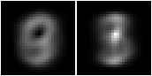
Imaging the 4 states ordered by size descending, $A\%X$,
pp = list(reversed(list(sset([(b,a) for (a,b) in aall(araa(uu,hrred(hr,xx)))]))))[:20]

[int(a) for (a,b) in pp]
# [2489, 2276, 1612, 1123]

bmwrite(file,bmhstack([bmborder(1,hrbm(28,1,2,hrhrred(hrhrsel(hr,aahr(uu,single(ss,1))),vvk))) for (_,ss) in pp]))
This 2-tuple is quite good at distinguishing between zero and non-zero.
5-tuple
Continue on to the 5-tuple,
(kmax,omax,qmax) = (5, 10, 10)

ll = buildcondrr(vvl,hr,kmax,omax,qmax)

rpln(ll)
# (1.4364854557895472, {<13,15>, <16,15>, <20,12>, <22,10>, <24,13>})
# (1.4388436113405096, {<13,15>, <16,15>, <20,12>, <22,10>, <24,14>})
# (1.4468132285301594, {<11,18>, <13,15>, <16,15>, <20,12>, <22,10>})
# (1.4474427280733204, {<14,15>, <17,15>, <20,12>, <22,10>, <24,13>})
# (1.4497701554712141, {<13,15>, <16,15>, <20,12>, <22,11>, <24,13>})
# (1.4500235885928272, {<13,15>, <16,15>, <20,12>, <22,10>, <24,12>})
# (1.4500244514704015, {<14,15>, <17,15>, <20,12>, <22,10>, <24,14>})
# (1.4505181754063234, {<13,10>, <13,15>, <16,15>, <20,12>, <22,10>})
# (1.4513236794288678, {<13,18>, <14,15>, <17,15>, <20,12>, <22,10>})
# (1.4522048769374534, {<10,18>, <13,15>, <16,15>, <20,12>, <22,10>})

rpln(reversed(list(sset([(algn(aa1)-algn(aar1),xx) for (e,xx) in ll for aa1 in [hhaa(hrhh(uu,hrhrred(hr,xx)))] for aar1 in [hhaa(hrhh(uu,hrhrred(hrr,xx)))]]))))
# (809.1235861373134, {<13,15>, <16,15>, <20,12>, <22,11>, <24,13>})
# (761.3003323882876, {<13,15>, <16,15>, <20,12>, <22,10>, <24,12>})
# (738.2133736383839, {<14,15>, <17,15>, <20,12>, <22,10>, <24,13>})
# (654.084544972684, {<13,18>, <14,15>, <17,15>, <20,12>, <22,10>})
# (644.4760839724622, {<13,15>, <16,15>, <20,12>, <22,10>, <24,13>})
# (635.2692466666049, {<14,15>, <17,15>, <20,12>, <22,10>, <24,14>})
# (545.3690945639028, {<13,15>, <16,15>, <20,12>, <22,10>, <24,14>})
# (518.1784362895924, {<11,18>, <13,15>, <16,15>, <20,12>, <22,10>})
# (485.09913398818026, {<13,10>, <13,15>, <16,15>, <20,12>, <22,10>})
# (444.6161086489592, {<10,18>, <13,15>, <16,15>, <20,12>, <22,10>})

rpln(reversed(list(sset([(rent(aa1,vaar1),xx) for (e,xx) in ll for aa1 in [hhaa(hrhh(uu,hrhrred(hr,xx)))] for vaar1 in [vsize(uu,xx,hhaa(hrhh(uu,hrhrred(hrr,xx))))]]))))
# (4.774342262630341, {<13,15>, <16,15>, <20,12>, <22,11>, <24,13>})
# (4.0464595839425925, {<14,15>, <17,15>, <20,12>, <22,10>, <24,13>})
# (3.7596434702714703, {<13,15>, <16,15>, <20,12>, <22,10>, <24,12>})
# (3.476669866227809, {<13,15>, <16,15>, <20,12>, <22,10>, <24,13>})
# (3.319595401602726, {<14,15>, <17,15>, <20,12>, <22,10>, <24,14>})
# (3.128531073666281, {<13,18>, <14,15>, <17,15>, <20,12>, <22,10>})
# (2.7186977082315025, {<13,15>, <16,15>, <20,12>, <22,10>, <24,14>})
# (2.5047556018341055, {<11,18>, <13,15>, <16,15>, <20,12>, <22,10>})
# (2.193180240754927, {<13,10>, <13,15>, <16,15>, <20,12>, <22,10>})
# (2.0803431289901795, {<10,18>, <13,15>, <16,15>, <20,12>, <22,10>})

xx = ll[0][1]

len(xx)
5

hrlent(uu,hr,xx,vvl)
1.4364854557895472

vol(uu,xx)
32

size(mul(hhaa(hrhh(uu,hrhrred(hrq,xx))),eff(hhaa(hrhh(uu,hrhrred(hr,xx))))))
# 1000 % 1

rpln(aall(araa(uu,hrred(hr,xx|vvl))))
# ({(digit, 0), (<13,15>, 0), (<16,15>, 0), (<20,12>, 0), (<22,10>, 0), (<24,13>, 0)}, 36 % 1)
# ({(digit, 0), (<13,15>, 0), (<16,15>, 0), (<20,12>, 0), (<22,10>, 0), (<24,13>, 1)}, 79 % 1)
# ({(digit, 0), (<13,15>, 0), (<16,15>, 0), (<20,12>, 0), (<22,10>, 1), (<24,13>, 0)}, 103 % 1)
# ...
# ({(digit, 9), (<13,15>, 1), (<16,15>, 1), (<20,12>, 1), (<22,10>, 0), (<24,13>, 1)}, 1 % 1)
# ({(digit, 9), (<13,15>, 1), (<16,15>, 1), (<20,12>, 1), (<22,10>, 1), (<24,13>, 0)}, 1 % 1)
# ({(digit, 9), (<13,15>, 1), (<16,15>, 1), (<20,12>, 1), (<22,10>, 1), (<24,13>, 1)}, 0 % 1)

bmwrite(file,bmborder(1,bmmax(hrbmav,0,0,hrbm(28,3,2,qqhr(2,uu,vvk,xx)))))

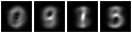
Imaging the first 20 states ordered by size descending, $\mathrm{top}(20)(A\%X)$,
pp = list(reversed(list(sset([(b,a) for (a,b) in aall(araa(uu,hrred(hr,xx)))]))))[:20]

[int(a) for (a,b) in pp]
# [898, 861, 673, 436, 407, 369, 359, 333, 299, 290, 245, 232, 217, 178, 169, 152, 150, 141, 133, 129]

bmwrite(file,bmhstack([bmborder(1,hrbm(28,1,2,hrhrred(hrhrsel(hr,aahr(uu,single(ss,1))),vvk))) for (_,ss) in pp]))

Let us apply the 5-tuple to the test sample to calculate the accuracy of prediction, \[ \{(Q\%V_{\mathrm{l}},~\mathrm{max}(R)) : (S,\cdot) \in A_{\mathrm{te}},~Q = \{S\}^{\mathrm{U}},~R = A * (Q\%X),~\mathrm{size}(R) > 0\} \]
def aarr(aa):
    return [(ss,float(q)) for (ss,q) in aall(aa)]

def amax(aa):
    ll = aall(norm(trim(aa)))
    ll.sort(key = lambda x: x[1], reverse = True)
    return llaa(ll[:1])

rpln([(aarr(red(qq,vvl)), aarr(amax(rr))) for hr1 in [hrhrred(hr,xx|vvl)] for (_,ss) in hhll(hrhh(uu,hrhrred(hrq,xx|vvl))) for qq in [single(ss,1)] for rr in[araa(uu,hrred(hrhrsel(hr1,hhhr(uu,aahh(red(qq,xx)))),vvl))] if size(rr) > 0][:20])
# ([({(digit, 7)}, 1.0)], [({(digit, 7)}, 0.4151376146788991)])
# ([({(digit, 0)}, 1.0)], [({(digit, 0)}, 0.7764127764127764)])
# ([({(digit, 9)}, 1.0)], [({(digit, 3)}, 0.49310344827586206)])
# ([({(digit, 3)}, 1.0)], [({(digit, 3)}, 0.49310344827586206)])
# ([({(digit, 1)}, 1.0)], [({(digit, 1)}, 0.6939078751857355)])
# ([({(digit, 6)}, 1.0)], [({(digit, 6)}, 0.6128133704735376)])
# ([({(digit, 7)}, 1.0)], [({(digit, 7)}, 0.35423925667828104)])
# ([({(digit, 7)}, 1.0)], [({(digit, 7)}, 0.4151376146788991)])
# ([({(digit, 7)}, 1.0)], [({(digit, 7)}, 0.35423925667828104)])
# ([({(digit, 3)}, 1.0)], [({(digit, 3)}, 0.49310344827586206)])
# ([({(digit, 6)}, 1.0)], [({(digit, 6)}, 0.6128133704735376)])
# ([({(digit, 8)}, 1.0)], [({(digit, 1)}, 0.6939078751857355)])
# ([({(digit, 5)}, 1.0)], [({(digit, 8)}, 0.4883720930232558)])
# ([({(digit, 6)}, 1.0)], [({(digit, 6)}, 0.6128133704735376)])
# ([({(digit, 6)}, 1.0)], [({(digit, 6)}, 0.4624624624624625)])
# ([({(digit, 9)}, 1.0)], [({(digit, 4)}, 0.4298440979955457)])
# ([({(digit, 4)}, 1.0)], [({(digit, 4)}, 0.4298440979955457)])
# ([({(digit, 4)}, 1.0)], [({(digit, 4)}, 0.4298440979955457)])
# ([({(digit, 1)}, 1.0)], [({(digit, 1)}, 0.6939078751857355)])
# ([({(digit, 1)}, 1.0)], [({(digit, 8)}, 0.47368421052631576)])
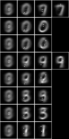
We show the test sample digit on the left and the best guess by the tuple on the right, along with the probability. In this case all 20 queries are effective and the model is correct 15 times.
These are the query images side by side with the slice for the tuple state,
bmwrite(file,bmvstack([bmhstack([bmborder(1,hrbm(28,1,2,hrhrred(hrev([i],hrq),vvk))), bmborder(1,hrbm(28,1,2,hrhrred(hrhrsel(hr,qq),vvk)))]) for i in range(min(20,hrsize(hrq))) for qq in [ hrhrred(hrev([i],hrq),xx)]]))
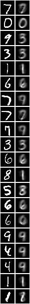
Overall, this model is correct for 44.8% of the test sample, \[ |\{R : (S,\cdot) \in A_{\mathrm{te}},~Q = \{S\}^{\mathrm{U}},~R = A * (Q\%X),~\mathrm{size}(\mathrm{max}(R) * (Q\%V_{\mathrm{l}})) > 0\}| \]
len([rr for hr1 in [hrhrred(hr,xx|vvl)] for (_,ss) in hhll(hrhh(uu,hrhrred(hrq,xx|vvl))) for qq in [single(ss,1)] for rr in [araa(uu,hrred(hrhrsel(hr1,hhhr(uu,aahh(red(qq,xx)))),vvl))] if size(rr) > 0 and size(mul(amax(rr),red(qq,vvl))) > 0])
448
12-tuple
Continue on to the 12-tuple,
(kmax,omax,qmax) = (12, 10, 10)

ll = buildcondrr(vvl,hr,kmax,omax,qmax)

rpln(ll)
# (0.4487613840558877, {<8,15>, <10,17>, <10,19>, <13,15>, <15,12>, <15,18>, <16,15>, <17,11>, <20,12>, <21,14>, <22,10>, <24,13>})
# (0.4488059178689614, {<8,15>, <10,17>, <10,19>, <13,15>, <15,12>, <15,18>, <16,15>, <17,12>, <20,12>, <21,14>, <22,10>, <24,13>})
# (0.4494382758230282, {<8,15>, <10,12>, <10,17>, <10,19>, <13,15>, <15,12>, <16,15>, <16,18>, <20,12>, <21,14>, <22,10>, <24,13>})
# (0.44971065389324316, {<8,15>, <10,17>, <10,19>, <13,15>, <15,12>, <16,15>, <16,18>, <17,12>, <20,12>, <21,14>, <22,10>, <24,13>})
# (0.45027981903127845, {<8,15>, <10,17>, <10,19>, <13,15>, <15,12>, <16,15>, <16,18>, <17,11>, <20,12>, <21,14>, <22,10>, <24,13>})
# (0.4507996248395969, {<8,15>, <9,12>, <10,17>, <10,19>, <13,15>, <15,12>, <16,15>, <16,18>, <20,12>, <21,14>, <22,10>, <24,13>})
# (0.45103768071372485, {<8,15>, <9,12>, <10,17>, <10,19>, <13,15>, <15,12>, <15,18>, <16,15>, <20,12>, <21,14>, <22,10>, <24,13>})
# (0.4513929339823175, {<6,16>, <8,15>, <10,12>, <10,17>, <13,15>, <14,18>, <15,12>, <16,15>, <20,12>, <21,14>, <22,10>, <24,13>})
# (0.4519764035368272, {<8,15>, <10,17>, <10,19>, <11,11>, <13,15>, <15,12>, <16,15>, <16,18>, <20,12>, <21,14>, <22,10>, <24,13>})
# (0.45260335677474206, {<8,15>, <10,12>, <10,17>, <10,19>, <13,15>, <15,12>, <16,15>, <17,18>, <20,12>, <21,14>, <22,10>, <24,13>})

rpln(reversed(list(sset([(algn(aa1)-algn(aar1),xx) for (e,xx) in ll for aa1 in [hhaa(hrhh(uu,hrhrred(hr,xx)))] for aar1 in [hhaa(hrhh(uu,hrhrred(hrr,xx)))]]))))
# (4710.191507206356, {<8,15>, <10,17>, <10,19>, <13,15>, <15,12>, <15,18>, <16,15>, <17,12>, <20,12>, <21,14>, <22,10>, <24,13>})
# (4636.906168187812, {<8,15>, <10,17>, <10,19>, <13,15>, <15,12>, <16,15>, <16,18>, <17,12>, <20,12>, <21,14>, <22,10>, <24,13>})
# (4608.906023772407, {<6,16>, <8,15>, <10,12>, <10,17>, <13,15>, <14,18>, <15,12>, <16,15>, <20,12>, <21,14>, <22,10>, <24,13>})
# (4576.4995186228825, {<8,15>, <10,17>, <10,19>, <13,15>, <15,12>, <15,18>, <16,15>, <17,11>, <20,12>, <21,14>, <22,10>, <24,13>})
# (4531.506995784216, {<8,15>, <10,17>, <10,19>, <13,15>, <15,12>, <16,15>, <16,18>, <17,11>, <20,12>, <21,14>, <22,10>, <24,13>})
# (4236.4203341864, {<8,15>, <10,12>, <10,17>, <10,19>, <13,15>, <15,12>, <16,15>, <16,18>, <20,12>, <21,14>, <22,10>, <24,13>})
# (4194.578095661386, {<8,15>, <9,12>, <10,17>, <10,19>, <13,15>, <15,12>, <15,18>, <16,15>, <20,12>, <21,14>, <22,10>, <24,13>})
# (4167.738085738728, {<8,15>, <10,17>, <10,19>, <11,11>, <13,15>, <15,12>, <16,15>, <16,18>, <20,12>, <21,14>, <22,10>, <24,13>})
# (4153.255987348684, {<8,15>, <10,12>, <10,17>, <10,19>, <13,15>, <15,12>, <16,15>, <17,18>, <20,12>, <21,14>, <22,10>, <24,13>})
# (4111.164512216985, {<8,15>, <9,12>, <10,17>, <10,19>, <13,15>, <15,12>, <16,15>, <16,18>, <20,12>, <21,14>, <22,10>, <24,13>})

rpln(reversed(list(sset([(rent(aa1,vaar1),xx) for (e,xx) in ll for aa1 in [hhaa(hrhh(uu,hrhrred(hr,xx)))] for vaar1 in [vsize(uu,xx,hhaa(hrhh(uu,hrhrred(hrr,xx))))]]))))
# (3116.3158977611056, {<6,16>, <8,15>, <10,12>, <10,17>, <13,15>, <14,18>, <15,12>, <16,15>, <20,12>, <21,14>, <22,10>, <24,13>})
# (3031.3295981763586, {<8,15>, <10,17>, <10,19>, <13,15>, <15,12>, <15,18>, <16,15>, <17,12>, <20,12>, <21,14>, <22,10>, <24,13>})
# (3021.9528122990414, {<8,15>, <10,17>, <10,19>, <13,15>, <15,12>, <15,18>, <16,15>, <17,11>, <20,12>, <21,14>, <22,10>, <24,13>})
# (2987.500469231527, {<8,15>, <9,12>, <10,17>, <10,19>, <13,15>, <15,12>, <15,18>, <16,15>, <20,12>, <21,14>, <22,10>, <24,13>})
# (2971.8243864387005, {<8,15>, <10,17>, <10,19>, <13,15>, <15,12>, <16,15>, <16,18>, <17,11>, <20,12>, <21,14>, <22,10>, <24,13>})
# (2967.3902079584514, {<8,15>, <10,17>, <10,19>, <13,15>, <15,12>, <16,15>, <16,18>, <17,12>, <20,12>, <21,14>, <22,10>, <24,13>})
# (2907.8950152716643, {<8,15>, <9,12>, <10,17>, <10,19>, <13,15>, <15,12>, <16,15>, <16,18>, <20,12>, <21,14>, <22,10>, <24,13>})
# (2881.520925887762, {<8,15>, <10,17>, <10,19>, <11,11>, <13,15>, <15,12>, <16,15>, <16,18>, <20,12>, <21,14>, <22,10>, <24,13>})
# (2867.4392998626136, {<8,15>, <10,12>, <10,17>, <10,19>, <13,15>, <15,12>, <16,15>, <17,18>, <20,12>, <21,14>, <22,10>, <24,13>})
# (2853.6303096867705, {<8,15>, <10,12>, <10,17>, <10,19>, <13,15>, <15,12>, <16,15>, <16,18>, <20,12>, <21,14>, <22,10>, <24,13>})

xx = ll[0][1]

len(xx)
12

hrlent(uu,hr,xx,vvl)
0.4487613840558877

vol(uu,xx)
4096

size(mul(hhaa(hrhh(uu,hrhrred(hrq,xx))),eff(hhaa(hrhh(uu,hrhrred(hr,xx))))))
# 876 % 1

rpln(aall(araa(uu,hrred(hr,xx|vvl))))

bmwrite(file,bmborder(1,bmmax(hrbmav,0,0,hrbm(28,3,2,qqhr(2,uu,vvk,xx)))))

Imaging the first 20 states ordered by size descending, $\mathrm{top}(20)(A\%X)$,
pp = list(reversed(list(sset([(b,a) for (a,b) in aall(araa(uu,hrred(hr,xx)))]))))[:20]

[int(a) for (a,b) in pp]
# [162, 138, 88, 72, 65, 64, 63, 55, 51, 45, 44, 44, 44, 44, 44, 42, 40, 36, 36, 35]

bmwrite(file,bmhstack([bmborder(1,hrbm(28,1,2,hrhrred(hrhrsel(hr,aahr(uu,single(ss,1))),vvk))) for (_,ss) in pp]))

We can see that as the tuple cardinality increases and the label entropy decreases, the slices are increasingly identifiable as a digit.
Let us apply the 12-tuple to the test sample to calculate the accuracy of prediction, \[ \{(Q\%V_{\mathrm{l}},~\mathrm{max}(R)) : (S,\cdot) \in A_{\mathrm{te}},~Q = \{S\}^{\mathrm{U}},~R = A * (Q\%X),~\mathrm{size}(R) > 0\} \]
rpln([(aarr(red(qq,vvl)), aarr(amax(rr))) for hr1 in [hrhrred(hr,xx|vvl)] for (_,ss) in hhll(hrhh(uu,hrhrred(hrq,xx|vvl))) for qq in [single(ss,1)] for rr in[araa(uu,hrred(hrhrsel(hr1,hhhr(uu,aahh(red(qq,xx)))),vvl))] if size(rr) > 0][:20])
# ([({(digit, 7)}, 1.0)], [({(digit, 7)}, 0.9777777777777777)])
# ([({(digit, 0)}, 1.0)], [({(digit, 0)}, 0.7818181818181819)])
# ([({(digit, 9)}, 1.0)], [({(digit, 9)}, 0.8)])
# ([({(digit, 3)}, 1.0)], [({(digit, 3)}, 0.875)])
# ([({(digit, 1)}, 1.0)], [({(digit, 1)}, 0.9814814814814815)])
# ([({(digit, 6)}, 1.0)], [({(digit, 6)}, 0.9722222222222222)])
# ([({(digit, 7)}, 1.0)], [({(digit, 7)}, 0.7894736842105263)])
# ([({(digit, 7)}, 1.0)], [({(digit, 7)}, 0.6)])
# ([({(digit, 7)}, 1.0)], [({(digit, 4)}, 0.8666666666666667)])
# ([({(digit, 3)}, 1.0)], [({(digit, 3)}, 0.6666666666666666)])
# ([({(digit, 6)}, 1.0)], [({(digit, 6)}, 1.0)])
# ([({(digit, 8)}, 1.0)], [({(digit, 4)}, 1.0)])
# ([({(digit, 5)}, 1.0)], [({(digit, 5)}, 1.0)])
# ([({(digit, 6)}, 1.0)], [({(digit, 6)}, 0.9722222222222222)])
# ([({(digit, 6)}, 1.0)], [({(digit, 6)}, 1.0)])
# ([({(digit, 9)}, 1.0)], [({(digit, 9)}, 0.782608695652174)])
# ([({(digit, 4)}, 1.0)], [({(digit, 4)}, 0.967741935483871)])
# ([({(digit, 4)}, 1.0)], [({(digit, 4)}, 0.8095238095238095)])
# ([({(digit, 1)}, 1.0)], [({(digit, 1)}, 0.9710144927536232)])
# ([({(digit, 1)}, 1.0)], [({(digit, 1)}, 0.8333333333333334)])
In this case all 20 queries are effective and the model is correct 18 times,
bmwrite(file,bmvstack([bmhstack([bmborder(1,hrbm(28,1,2,hrhrred(hrev([i],hrq),vvk))), bmborder(1,hrbm(28,1,2,hrhrred(hrhrsel(hr,qq),vvk)))]) for i in range(min(20,hrsize(hrq))) for qq in [hrhrred(hrev([i],hrq),xx)]]))
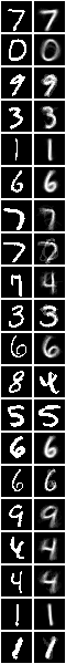
Overall, this model is correct for 59.6% of the test sample,
len([rr for hr1 in [hrhrred(hr,xx|vvl)] for (_,ss) in hhll(hrhh(uu,hrhrred(hrq,xx|vvl))) for qq in [single(ss,1)] for rr in [araa(uu,hrred(hrhrsel(hr1,hhhr(uu,aahh(red(qq,xx)))),vvl))] if size(rr) > 0 and size(mul(amax(rr),red(qq,vvl))) > 0])
596
The prediction accuracy of larger tuples is not likely to be much higher, because the query effectiveness declines as the tuple cardinality increases.
1-tuple 15-fud
Instead of determining minimum subsets of the query variables that are causal or predictive by using the conditional entropy tuple set builder, consider using the conditional entropy fud decomper, $\{D\} = \mathrm{leaves}(\mathrm{tree}(Z_{P,A,\mathrm{L,D,F}}))$.
The resultant decomposition consists of singleton fuds of self partition transforms of smaller tuples. In this way a set of paths of different tuples for different slices can reduce the label entropy,
def decompercondrr(ll,uu,aa,kmax,omax,fmax):
    return parametersSystemsHistoryRepasDecomperConditionalFmaxRepa(kmax,omax,fmax,uu,ll,aa)

(kmax,omax) = (1,5)

(uu1,df) = decompercondrr(vvl,uu,hr,kmax,omax,15)

dfund(df)
# {<6,16>, <8,11>, <8,15>, <9,18>, <11,11>, <13,15>, <15,12>, <15,14>, <16,10>, <16,16>, <17,13>, <17,15>, <19,11>, <20,12>, <22,10>}

len(dfund(df))
15

def dfll(df):
    return treesPaths(dfzz(df))

rpln([[fund(ff) for (_,ff) in ll] for ll in dfll(df)])
# [{<13,15>}, {<22,10>}, {<20,12>}, {<16,10>}, {<15,14>}, {<17,13>}, {<6,16>}]
# [{<13,15>}, {<22,10>}, {<20,12>}, {<16,10>}, {<8,15>}]
# [{<13,15>}, {<22,10>}, {<20,12>}, {<9,18>}]
# [{<13,15>}, {<22,10>}, {<16,16>}]
# [{<13,15>}, {<17,15>}, {<19,11>}, {<11,11>}]
# [{<13,15>}, {<17,15>}, {<8,11>}, {<15,12>}]
Now analyse with the fud decomposition fud, $F = D^{\mathrm{F}}$, (see Practicable fud decomposition fud),
ff = dfnul(uu1,df,1)

uu2 = uunion(uu,fsys(ff))

hrb = hrfmul(uu2,ff,hr)
The label entropy, $\mathrm{lent}(A * \mathrm{his}(F^{\mathrm{T}}),W_F,V_{\mathrm{l}})$, where $W_F = \mathrm{der}(F)$, is
hrlent(uu2,hrb,fder(ff),vvl)
1.4172761780693333
Imaging the underlying $V_F = \mathrm{und}(F)$ overlaid on the average, $\hat{A}\%V_{\mathrm{k}}$,
bmwrite(file,bmborder(1,bmmax(hrbmav,0,0,hrbm(28,3,2,qqhr(2,uu,vvk,fund(ff))))))

We can see that a decomposition limited to 15 fuds has an expected path length of 4 but a label entropy similar to the 5-tuple above. Only 3 of the variables are in both models,
xx = sset(map(stringsVariable,["<13,15>","<16,15>","<20,12>","<22,10>","<24,13>"]))

dfund(df) & xx
# {<13,15>, <20,12>, <22,10>}
The conditional entropy decomposition fud of a bi-valent substrate is always effective, $\mathrm{size}((A_{\mathrm{te}} * F^{\mathrm{T}}) * (A * F^{\mathrm{T}})^{\mathrm{F}}) = \mathrm{size}(A_{\mathrm{te}})$, effective,
hrqb = hrfmul(uu2,ff,hrq)

size(mul(hhaa(hrhh(uu2,hrhrred(hrqb,fder(ff)))),eff(hhaa(hrhh(uu2,hrhrred(hrb,fder(ff)))))))
# 1000 % 1
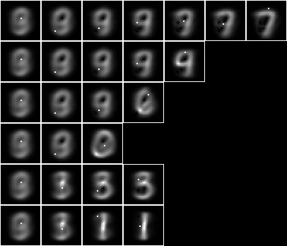
Imaging the slices of the decomposition,
pp = treesPaths(hrmult(uu1,df,hr))

rpln([[hrsize(hr) for (_,hr) in ll] for ll in pp])
# [7500, 4765, 3406, 2564, 1569, 1130, 811]
# [7500, 4765, 3406, 2564, 995]
# [7500, 4765, 3406, 842]
# [7500, 4765, 1359]
# [7500, 2735, 1441, 1070]
# [7500, 2735, 1294, 984]

bmwrite(file,ppbm(uu,vvk,28,2,2,pp))
Let us apply the 15-fud to the test sample to calculate the accuracy of prediction, \[ \begin{eqnarray} &&\{(Q\%V_{\mathrm{l}},~\mathrm{max}(R)) : (S,\cdot) \in A_{\mathrm{te}} * \mathrm{his}(F^{\mathrm{T}})~\%~(W_F \cup V_{\mathrm{l}}),~Q = \{S\}^{\mathrm{U}}, \\ &&\hspace{8em}R = A * \mathrm{his}(F^{\mathrm{T}})~\%~(W_F \cup V_{\mathrm{l}}) * (Q\%W_F),~\mathrm{size}(R) > 0\} \end{eqnarray} \]
rpln([(aarr(red(qq,vvl)), aarr(amax(rr))) for hr1 in [hrhrred(hrb,fder(ff)|vvl)] for (_,ss) in hhll(hrhh(uu2,hrhrred(hrqb,fder(ff)|vvl))) for qq in [single(ss,1)] for rr in [araa(uu2,hrred(hrhrsel(hr1,hhhr(uu2,aahh(red(qq,fder(ff))))),vvl))] if size(rr) > 0][:20])
# ([({(digit, 7)}, 1.0)], [({(digit, 7)}, 0.7174825174825175)])
# ([({(digit, 0)}, 1.0)], [({(digit, 0)}, 0.6117353308364545)])
# ([({(digit, 9)}, 1.0)], [({(digit, 5)}, 0.3783783783783784)])
# ([({(digit, 3)}, 1.0)], [({(digit, 3)}, 0.5753052917232022)])
# ([({(digit, 1)}, 1.0)], [({(digit, 1)}, 0.8231780167264038)])
# ([({(digit, 6)}, 1.0)], [({(digit, 6)}, 0.6442141623488774)])
# ([({(digit, 7)}, 1.0)], [({(digit, 7)}, 0.7174825174825175)])
# ([({(digit, 7)}, 1.0)], [({(digit, 7)}, 0.7174825174825175)])
# ([({(digit, 7)}, 1.0)], [({(digit, 4)}, 0.6975524475524476)])
# ([({(digit, 3)}, 1.0)], [({(digit, 3)}, 0.5753052917232022)])
# ([({(digit, 6)}, 1.0)], [({(digit, 6)}, 0.6442141623488774)])
# ([({(digit, 8)}, 1.0)], [({(digit, 3)}, 0.5753052917232022)])
# ([({(digit, 5)}, 1.0)], [({(digit, 3)}, 0.5753052917232022)])
# ([({(digit, 6)}, 1.0)], [({(digit, 6)}, 0.6442141623488774)])
# ([({(digit, 6)}, 1.0)], [({(digit, 6)}, 0.6442141623488774)])
# ([({(digit, 9)}, 1.0)], [({(digit, 9)}, 0.5602836879432624)])
# ([({(digit, 4)}, 1.0)], [({(digit, 4)}, 0.29153605015673983)])
# ([({(digit, 4)}, 1.0)], [({(digit, 4)}, 0.29153605015673983)])
# ([({(digit, 1)}, 1.0)], [({(digit, 1)}, 0.8231780167264038)])
# ([({(digit, 1)}, 1.0)], [({(digit, 1)}, 0.8231780167264038)])
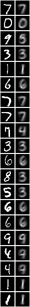
In this case all 20 queries are effective and the model is correct 16 times,
bmwrite(file,bmvstack([bmhstack([bmborder(1,hrbm(28,1,2,hrhrred(hrev([i],hrqb),vvk))), bmborder(1,hrbm(28,1,2,hrhrred(hrhrsel(hrb,qq),vvk)))]) for i in range(min(20,hrsize(hrqb))) for qq in [hrhrred(hrev([i],hrqb),fder(ff))]]))
Overall, this model is correct for 56.7% of the test sample,
len([rr for hr1 in [hrhrred(hrb,fder(ff)|vvl)] for (_,ss) in hhll(hrhh(uu2,hrhrred(hrqb,fder(ff)|vvl))) for qq in [single(ss,1)] for rr in [araa(uu2,hrred(hrhrsel(hr1,hhhr(uu2,aahh(red(qq,fder(ff))))),vvl))] if size(rr) > 0 and size(mul(amax(rr),red(qq,vvl))) > 0])
567
This is considerably more accurate than the 5-tuple (44.8%). It is approaching the accuracy of the 12-tuple (60.0%).
1-tuple 127-fud
Increasing the decomposition fuds cardinality to an expected path length of 7,
(uu1,df) = decompercondrr(vvl,uu,hr,kmax,omax,127)

len(dfund(df))
101

rpln([[fund(ff) for (_,ff) in ll] for ll in dfll(df)])
# [{<13,15>}, {<22,10>}, {<20,12>}, {<16,10>}, {<15,14>}, {<17,13>}, {<6,16>}, {<18,9>}, {<10,19>}, {<11,17>}, {<21,15>}, {<24,14>}]
# [{<13,15>}, {<22,10>}, {<20,12>}, {<16,10>}, {<15,14>}, {<17,13>}, {<6,16>}, {<18,9>}, {<10,19>}, {<11,17>}, {<15,15>}, {<6,11>}, {<13,10>}]
# [{<13,15>}, {<22,10>}, {<20,12>}, {<16,10>}, {<15,14>}, {<17,13>}, {<6,16>}, {<18,9>}, {<10,19>}, {<20,8>}, {<16,13>}, {<14,14>}]
# ...
# [{<13,15>}, {<17,15>}, {<8,11>}, {<12,10>}, {<19,12>}, {<19,15>}]
# [{<13,15>}, {<17,15>}, {<8,11>}, {<12,10>}, {<19,12>}, {<12,13>}]
# [{<13,15>}, {<17,15>}, {<8,11>}, {<12,10>}, {<24,16>}]

ff = dfnul(uu1,df,1)

uu2 = uunion(uu,fsys(ff))

hrb = hrfmul(uu2,ff,hr)

hrlent(uu2,hrb,fder(ff),vvl)
0.7456431103312635

bmwrite(file,bmborder(1,bmmax(hrbmav,0,0,hrbm(28,3,2,qqhr(2,uu,vvk,fund(ff))))))

Imaging the slices of the decomposition,
pp = treesPaths(hrmult(uu1,df,hr))

rpln([[hrsize(hr) for (_,hr) in ll] for ll in pp])
# [7500, 4765, 3406, 2564, 1569, 1130, 811, 715, 651, 241, 86, 52]
# [7500, 4765, 3406, 2564, 1569, 1130, 811, 715, 651, 241, 155, 128, 121]
# [7500, 4765, 3406, 2564, 1569, 1130, 811, 715, 651, 410, 401, 394]
# ...
# [7500, 2735, 1294, 310, 196, 114]
# [7500, 2735, 1294, 310, 196, 82]
# [7500, 2735, 1294, 310, 114]

bmwrite(file,ppbm(uu,vvk,28,1,2,pp))
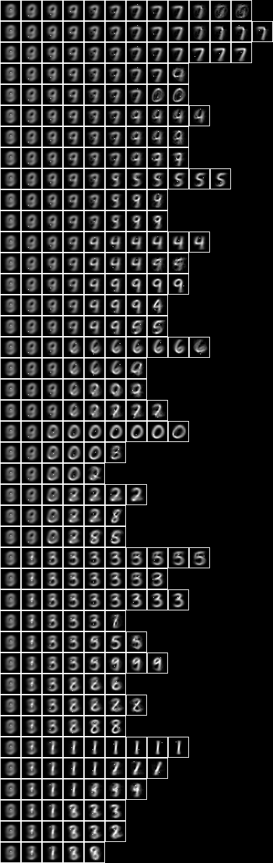
The decomposition fud is still effective,
hrqb = hrfmul(uu2,ff,hrq)

size(mul(hhaa(hrhh(uu2,hrhrred(hrqb,fder(ff)))),eff(hhaa(hrhh(uu2,hrhrred(hrb,fder(ff)))))))
# 1000 % 1
Let us apply the 127-fud to the test sample to calculate the accuracy of prediction,
rpln([(aarr(red(qq,vvl)), aarr(amax(rr))) for hr1 in [hrhrred(hrb,fder(ff)|vvl)] for (_,ss) in hhll(hrhh(uu2,hrhrred(hrqb,fder(ff)|vvl))) for qq in [single(ss,1)] for rr in [araa(uu2,hrred(hrhrsel(hr1,hhhr(uu2,aahh(red(qq,fder(ff))))),vvl))] if size(rr) > 0][:20])
# ([({(digit, 7)}, 1.0)], [({(digit, 7)}, 0.9639175257731959)])
# ([({(digit, 0)}, 1.0)], [({(digit, 0)}, 0.9884726224783862)])
# ([({(digit, 9)}, 1.0)], [({(digit, 9)}, 0.9090909090909091)])
# ([({(digit, 3)}, 1.0)], [({(digit, 3)}, 0.9798387096774194)])
# ([({(digit, 1)}, 1.0)], [({(digit, 1)}, 0.9855769230769231)])
# ([({(digit, 6)}, 1.0)], [({(digit, 6)}, 0.9707792207792207)])
# ([({(digit, 7)}, 1.0)], [({(digit, 7)}, 0.9047619047619048)])
# ([({(digit, 7)}, 1.0)], [({(digit, 7)}, 0.9639175257731959)])
# ([({(digit, 7)}, 1.0)], [({(digit, 5)}, 0.5238095238095238)])
# ([({(digit, 3)}, 1.0)], [({(digit, 3)}, 0.9798387096774194)])
# ([({(digit, 6)}, 1.0)], [({(digit, 6)}, 0.9707792207792207)])
# ([({(digit, 8)}, 1.0)], [({(digit, 3)}, 0.7954545454545454)])
# ([({(digit, 5)}, 1.0)], [({(digit, 5)}, 0.7876106194690266)])
# ([({(digit, 6)}, 1.0)], [({(digit, 6)}, 0.9707792207792207)])
# ([({(digit, 6)}, 1.0)], [({(digit, 6)}, 0.7721518987341772)])
# ([({(digit, 9)}, 1.0)], [({(digit, 9)}, 0.9184782608695652)])
# ([({(digit, 4)}, 1.0)], [({(digit, 4)}, 0.8055555555555556)])
# ([({(digit, 4)}, 1.0)], [({(digit, 4)}, 0.8055555555555556)])
# ([({(digit, 1)}, 1.0)], [({(digit, 1)}, 0.9855769230769231)])
# ([({(digit, 1)}, 1.0)], [({(digit, 1)}, 0.7833333333333333)])
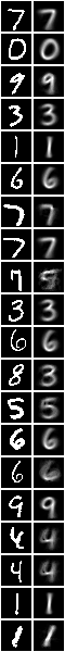
In this case all 20 queries are effective and the model is correct 18 times,
bmwrite(file,bmvstack([bmhstack([bmborder(1,hrbm(28,1,2,hrhrred(hrev([i],hrqb),vvk))), bmborder(1,hrbm(28,1,2,hrhrred(hrhrsel(hrb,qq),vvk)))]) for i in range(min(20,hrsize(hrqb))) for qq in [hrhrred(hrev([i],hrqb),fder(ff))]]))
Overall, this model is correct for 70.0% of the test sample,
len([rr for hr1 in [hrhrred(hrb,fder(ff)|vvl)] for (_,ss) in hhll(hrhh(uu2,hrhrred(hrqb,fder(ff)|vvl))) for qq in [single(ss,1)] for rr in [araa(uu2,hrred(hrhrsel(hr1,hhhr(uu2,aahh(red(qq,fder(ff))))),vvl))] if size(rr) > 0 and size(mul(amax(rr),red(qq,vvl))) > 0])
700
This is considerably more accurate than the 12-tuple (60.0%), which is also much less effective (87.6% instead of 100%).
1-tuple 511-fud
Increasing the decomposition fuds cardinality to an expected path length of 9,
(uu1,df) = decompercondrr(vvl,uu,hr,kmax,omax,511)

len(dfund(df))
236

ff = dfnul(uu1,df,1)

uu2 = uunion(uu,fsys(ff))

hrb = hrfmul(uu2,ff,hr)

hrlent(uu2,hrb,fder(ff),vvl)
0.2427582319997974

bmwrite(file,bmborder(1,bmmax(hrbmav,0,0,hrbm(28,3,2,qqhr(2,uu,vvk,fund(ff))))))

Overall, this model is correct for 75.5% of the test sample,
hrqb = hrfmul(uu2,ff,hrq)

len([rr for hr1 in [hrhrred(hrb,fder(ff)|vvl)] for (_,ss) in hhll(hrhh(uu2,hrhrred(hrqb,fder(ff)|vvl))) for qq in [single(ss,1)] for rr in [araa(uu2,hrred(hrhrsel(hr1,hhhr(uu2,aahh(red(qq,fder(ff))))),vvl))] if size(rr) > 0 and size(mul(amax(rr),red(qq,vvl))) > 0])
755
2-tuple 15-fud
Now consider a 2-tuple for each fud in a 15-fud decomposition,
(kmax,omax) = (2,5)

(uu1,df) = decompercondrr(vvl,uu,hr,kmax,omax,15)

len(dfund(df))
29

rpln([[fund(ff) for (_,ff) in ll] for ll in dfll(df)])
# [{<14,15>, <17,15>}, {<21,12>, <23,11>}, {<16,13>, <19,13>}, {<7,15>, <10,15>}]
# [{<14,15>, <17,15>}, {<21,12>, <23,11>}, {<12,15>, <15,15>}]
# [{<14,15>, <17,15>}, {<21,12>, <23,11>}, {<10,19>, <17,17>}]
# [{<14,15>, <17,15>}, {<21,13>, <24,12>}, {<8,15>, <21,11>}, {<13,17>, <14,19>}]
# [{<14,15>, <17,15>}, {<21,13>, <24,12>}, {<9,19>, <13,11>}]
# [{<14,15>, <17,15>}, {<19,11>, <24,13>}, {<19,13>, <22,13>}]
# [{<14,15>, <17,15>}, {<19,11>, <24,13>}, {<11,16>, <11,18>}]
# [{<14,15>, <17,15>}, {<11,11>, <20,11>}, {<8,11>, <16,12>}]

ff = dfnul(uu1,df,1)

uu2 = uunion(uu,fsys(ff))

hrb = hrfmul(uu2,ff,hr)

hrlent(uu2,hrb,fder(ff),vvl)
1.1776004502299107

bmwrite(file,bmborder(1,bmmax(hrbmav,0,0,hrbm(28,3,2,qqhr(2,uu,vvk,fund(ff))))))

The decomposition fud is still effective,
hrqb = hrfmul(uu2,ff,hrq)

size(mul(hhaa(hrhh(uu2,hrhrred(hrqb,fder(ff)))),eff(hhaa(hrhh(uu2,hrhrred(hrb,fder(ff)))))))
# 1000 % 1
Imaging the slices of the decomposition,
pp = treesPaths(hrmult(uu1,df,hr))

rpln([[hrsize(hr) for (_,hr) in ll] for ll in pp])
# [7500, 2250, 1008, 618]
# [7500, 2250, 614]
# [7500, 2250, 368]
# [7500, 1913, 979, 386]
# [7500, 1913, 498]
# [7500, 1693, 578]
# [7500, 1693, 660]
# [7500, 1644, 988]

bmwrite(file,ppbm(uu,vvk,28,2,2,pp))
Overall, this model is correct for 58% of the test sample,
len([rr for hr1 in [hrhrred(hrb,fder(ff)|vvl)] for (_,ss) in hhll(hrhh(uu2,hrhrred(hrqb,fder(ff)|vvl))) for qq in [single(ss,1)] for rr in [araa(uu2,hrred(hrhrsel(hr1,hhhr(uu2,aahh(red(qq,fder(ff))))),vvl))] if size(rr) > 0 and size(mul(amax(rr),red(qq,vvl))) > 0])
580
So the accuracy is little better than the 15-mono-variate-fud (56.7%).
2-tuple 127-fud
Now consider a 2-tuple for each fud in a 127-fud decomposition,
(uu1,df) = decompercondrr(vvl,uu,hr,kmax,omax,127)

len(dfund(df))
153

rpln([[fund(ff) for (_,ff) in ll] for ll in dfll(df)])
# [{<14,15>, <17,15>}, {<21,12>, <23,11>}, {<16,13>, <19,13>}, {<7,15>, <10,15>}, {<8,15>, <17,12>}, {<6,13>, <15,14>}, {<5,14>, <12,13>}]
# [{<14,15>, <17,15>}, {<21,12>, <23,11>}, {<16,13>, <19,13>}, {<7,15>, <10,15>}, {<8,15>, <17,12>}, {<14,13>, <16,18>}]
# [{<14,15>, <17,15>}, {<21,12>, <23,11>}, {<16,13>, <19,13>}, {<7,15>, <10,15>}, {<14,13>, <22,8>}]
# ...
# [{<14,15>, <17,15>}, {<11,11>, <20,11>}, {<7,15>, <9,15>}, {<13,13>, <22,13>}]
# [{<14,15>, <17,15>}, {<11,11>, <20,11>}, {<7,15>, <9,15>}, {<11,15>, <22,14>}]
# [{<14,15>, <17,15>}, {<11,11>, <20,11>}, {<18,10>, <24,13>}]

ff = dfnul(uu1,df,1)

uu2 = uunion(uu,fsys(ff))

hrb = hrfmul(uu2,ff,hr)

hrlent(uu2,hrb,fder(ff),vvl)
0.46080763495801413

bmwrite(file,bmborder(1,bmmax(hrbmav,0,0,hrbm(28,3,2,qqhr(2,uu,vvk,fund(ff))))))

The decomposition fud is slightly ineffective,
hrqb = hrfmul(uu2,ff,hrq)

size(mul(hhaa(hrhh(uu2,hrhrred(hrqb,fder(ff)))),eff(hhaa(hrhh(uu2,hrhrred(hrb,fder(ff)))))))
# 999 % 1
Overall, this model is correct for 74.0% of the test sample,
len([rr for hr1 in [hrhrred(hrb,fder(ff)|vvl)] for (_,ss) in hhll(hrhh(uu2,hrhrred(hrqb,fder(ff)|vvl))) for qq in [single(ss,1)] for rr in [araa(uu2,hrred(hrhrsel(hr1,hhhr(uu2,aahh(red(qq,fder(ff))))),vvl))] if size(rr) > 0 and size(mul(amax(rr),red(qq,vvl))) > 0])
740
So the accuracy is better than the 127-mono-variate-fud (70.0%), but not as good as the 511-mono-variate-fud (75.5%).
3-tuple 127-fud
Finally, consider tri-variate-fuds,
(kmax,omax) = (3, 5)

(uu1,df) = decompercondrr(vvl,uu,hr,kmax,omax,127)

len(dfund(df))
205

ff = dfnul(uu1,df,1)

uu2 = uunion(uu,fsys(ff))

hrb = hrfmul(uu2,ff,hr)

hrlent(uu2,hrb,fder(ff),vvl)
0.26909954826249827

bmwrite(file,bmborder(1,bmmax(hrbmav,0,0,hrbm(28,3,2,qqhr(2,uu,vvk,fund(ff))))))

The decomposition fud is slightly ineffective,
hrqb = hrfmul(uu2,ff,hrq)

size(mul(hhaa(hrhh(uu2,hrhrred(hrqb,fder(ff)))),eff(hhaa(hrhh(uu2,hrhrred(hrb,fder(ff)))))))
# 994 % 1
Overall, this model is correct for 73.9% of the test sample,
len([rr for hr1 in [hrhrred(hrb,fder(ff)|vvl)] for (_,ss) in hhll(hrhh(uu2,hrhrred(hrqb,fder(ff)|vvl))) for qq in [single(ss,1)] for rr in [araa(uu2,hrred(hrhrsel(hr1,hhhr(uu2,aahh(red(qq,fder(ff))))),vvl))] if size(rr) > 0 and size(mul(amax(rr),red(qq,vvl))) > 0])
739
So the accuracy of the 127-tri-variate-fud is a little worse than that of the 127-bi-variate-fud (74.0%).
Overall, of all of these models the 511-mono-variate-fud has the highest accuracy of 75.5%.
To conclude, a model consisting of only substrate variables can have reasonable accuracy/effectiveness with respect to digit, considering that the relative entropy of a substrate model is always quite low compared to induced models.