MNIST - handwritten digits
Introduction
The MNIST dataset was constructed from NIST’s Special Database 3 and Special Database 1 which contain binary images of handwritten digits. The images consist of arrays of 28x28 pixel variables of valency 256 representing grey levels - 0 means background (black in images below), 255 means foreground (white in images below). There is also the digit variable of valency 10 with values from 0 to 9. The training dataset contains 60,000 events and the test dataset contains 10,000 events.
We shall analyse this dataset using the NISTPy repository which depends on the AlignmentRepaPy repository. The AlignmentRepaPy repository is a fast Python and C implementation of some of the practicable inducers described in the paper. The code in this section can be executed by copying and pasting the code into a Python interpreter, see README. Also see the Introduction in Notation.
Analysis
Properties of the sample regions
Predicting digit without modelling
Modelling
Summary
Substrate models
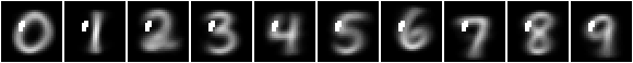
First, consider the properties of the sample. Here are some examples from the 28x28 pixel images of the training sample,

This is the average image,

Highly inter-dependent pixels in the images can be grouped together in sets or tuples. We can search for these highly aligned tuples and then repeat the search having subtracted the previous tuples. These are the first 12 tuples, shown with each tuple highlighted in the average image,


Here is the first tuple overlaid on the average for each digit,
We can see that the first tuple appears in the top loop where a three would differ from an eight.
A tuple can be thought of as a simple model of the sample. By this we mean that the tuple classifies the sample. Here are average images of the first 20 slices or image-groupings of the first tuple’s classification, in order of decreasing slice size,

The first slice is by far the largest. In this case all of the pixels of the tuple are background, so it includes all images where this region is blank. The remaining slices all have at least one foreground pixel in this region, for which there are images for most digits except one.
A tuple’s alignment is a measure of its likelihood as a model of the sample. Alignment is a statistic similar to mutual entropy which measures the degree of dependency between the variables within the model. The alignments of the first three tuples are 23,407, 22,974 and 23,104. The alignment the 12th tuple is lower, at 20,262. The union of the first 12 tuples is

The following tuples are more peripheral. The alignment of the 18th tuple is 18,202. The union of the first 18 tuples is

We can repeat this analysis for square regions of 10x10 pixels chosen randomly from the sample images. Again, the image regions can be averaged together,

In this case the first three tuples are,


The alignments are 22,033, 22,102 and 21,469.
The eighth and ninth tuples are,


The alignments rapidly decrease between the 8th and 9th tuples from 17,068 to 1,509.
Similarly, consider square regions of 11x11 pixels where the central pixel is always foreground chosen randomly from the sample images. The average centred square region image is,

In this case the first two tuples are,


The alignments are 23,769 and 23,109.
Induced models
Now consider unsupervised induced models. These are derived models of the relationships between the pixels of the images in the training sample. These models are more complex than the simple tuples above because they consist of derived variables.
Derived variables depend on underlying variables. They classify the values of their underlying variables into fewer derived values. We can induce a model by searching for tuples of derived variables that maximise alignment per derived value. The models are built bottom-up in layers of derived variables that depend directly or indirectly on the underlying pixels of the images. The highest layers have the highest derived value alignment.
In fact, this optimisation of alignment per derived value is too generalised to maximise the overall alignment of the model. So this search is repeated recursively to a create a model that consists of a tree of sub-models. Every node sub-model of the tree sees only a subset slice of the sample images. This slice depends on the path of its ancestor sub-models. The sub-models maximise the derived tuple alignments of the layers of derived variables that depend on the underlying pixels of the slice images. That is, the contingent sub-models specialise in particular slices and so the total alignment of the whole model is maximised.
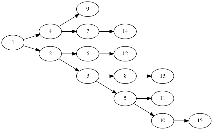
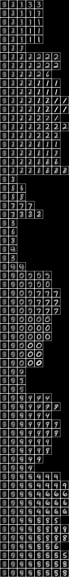
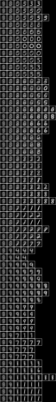
For example, this small model consists a tree of 15 sub-models,
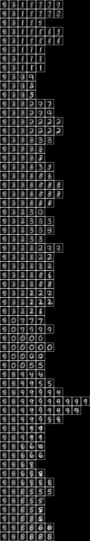
When we apply the model to the sample we can view the averaged slice image for each node,
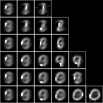
Here we have shown the model as a vertical stack of sub-model paths of averaged slice images. Each path runs horizontally from the root slice on the left to the leaf slice on the right. The underlying pixels of each node sub-model are also shown superimposed on each slice image. This shows where the ‘attention’ is during decomposition along a path.
This model depends on 134 underlying variables (pixels) of the 784 (= 28x28) in the images. Overall, the model has 515 variables. The alignment of the model is 137,828.
The leftmost column contains only the root slice, which is the entire sample. Here are the root underlying variables shown superimposed on the averaged root slice,

This tuple is similar to the most highly aligned tuple of the non-modelled case, above,
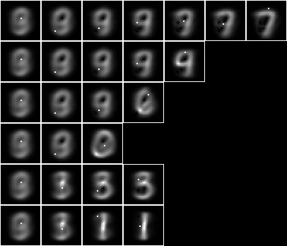
If we examine one of the derived variables in the highest layer of this root sub-model, we can see its underlying dependencies,
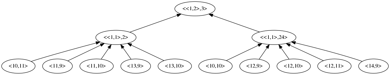
We can see that the bottom layer consists of pixel variables denoted by their coordinate. The root sub-model has two layers above this. The underlying variables are a subset of the root sub-model’s underlying,
# {<10,10>, <10,11>, <11,9>, <11,10>, <12,9>, <12,10>, <12,11>, <13,9>, <13,10>, <14,9>}

This derived variable has two values which classify the sample into two large slices,


These images are similar to those of sub-models 4 and 2 in the second column above.
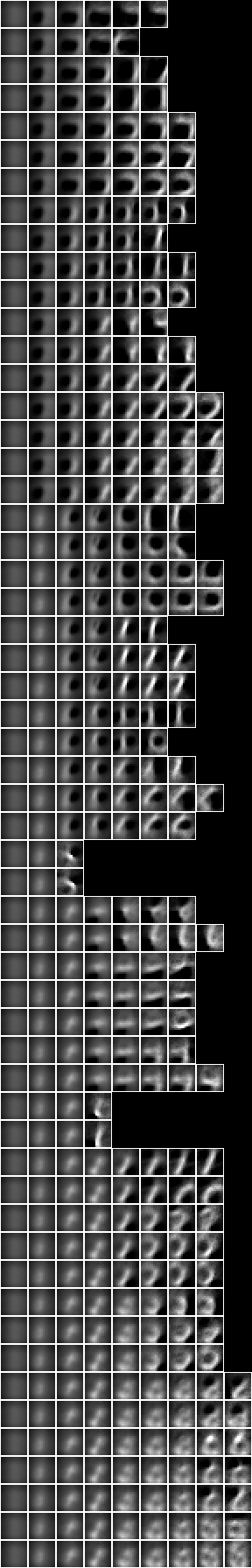
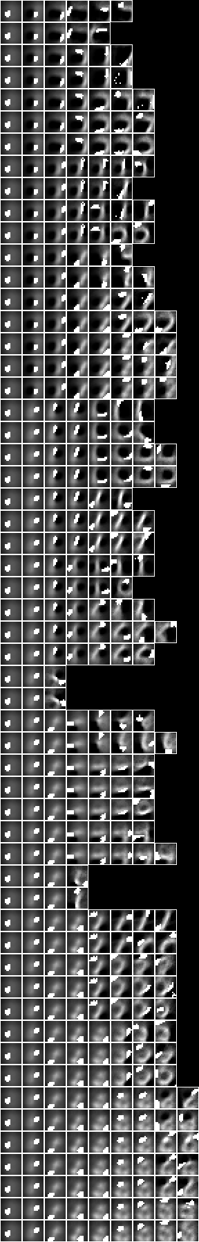
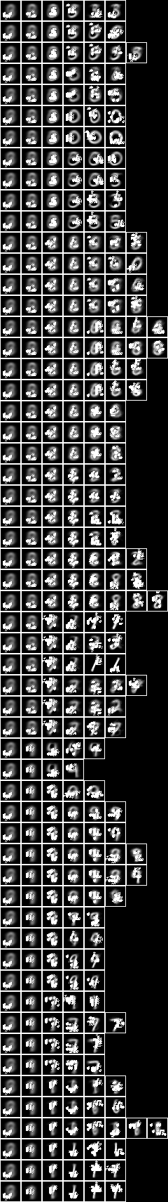
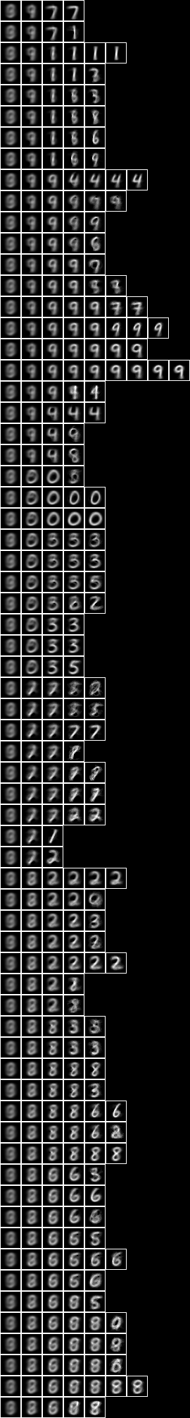
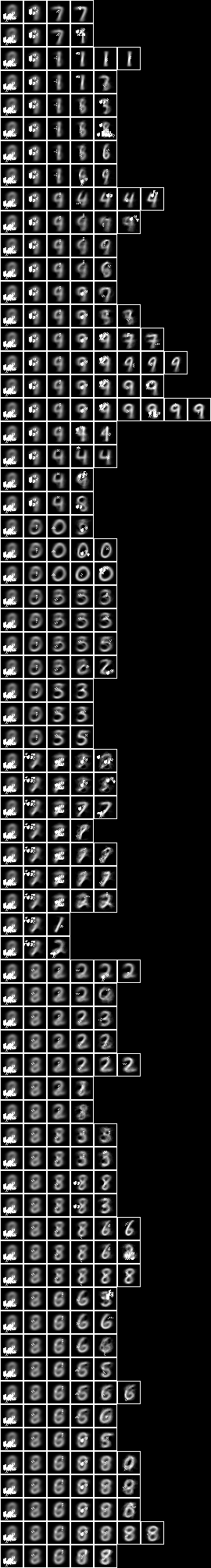
Now let us examine a larger model consisting of a tree of 127 sub-models. Below is an image of the decomposition slices, and adjacent is an image of the underlying variables superimposed on the slices,
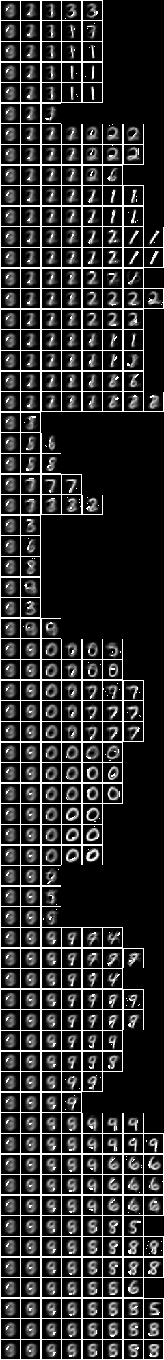
This model depends on 488 underlying variables. Overall, the model has 4040 variables. The alignment of the model is 132,688.
The root underlying variables are similar to those of the smaller model,

Now let us query the model with an image to see the slice in which it is classified. Choose, for example, this five,

Applying the model we find the average image of the leaf slice to be

We can see this leaf slice at the end of a three step path in the middle of the model above. Here are some of the slice images,

Although the most common digit in the slice is a five, we can see that there quite a lot of other similar looking digits.
Similarly, choosing this one,

we find the average leaf slice image to be

This leaf slice is at the end of the five steps of the third path in the model above. Here are the slice images,

In this case the leaf slice contains only ones.
If we apply this unsupervised model to a subset of 1000 images of the test sample we find that it correctly predicts or classifies the digit for 61.2% of them.
We can continue on to induce a model of square regions of 15x15 pixels chosen randomly from the sample images,
This regional model depends on all 225 (= 15x15) underlying variables. Overall, the model has 4082 variables. The alignment of the model is 195,132.
We can go on to create other regional models, such as square regions of 10x10 pixels (alignment 158,224), and centred square regions of 11x11 pixels (alignment 47,814).
Instead of building a model on a substrate of the pixels, consider a substrate that consists of the derived variables of copies of underlying regional models arranged regularly to cover the entire 28x28 pixels. Here is a two level model where the substrate of the upper level consists of 5x5 frames of the derived variables of the 15x15 pixel regional model,
This two level model depends on 595 of 784 (= 28x28) underlying variables. Overall, the model has 5787 variables. The alignment of the model is 174,749, which is higher than the one level model (132,688). That implies that this model is a more likely explanation of the data. We have, in effect, added our topological knowledge of the two dimension array of pixels to make a better, more global, model.
Predicting digit
While the alignment has increased considerably, the accuracy of predicting digit is not much different, at 61.0%. This is because the induced models are unsupervised with respect to the label, digit. That is, they have no access to digit, so the accuracy as a classifier depends solely on what is intrinsic in the relationships between pixels.
In order to consider this functional or causal relationship between the pixels variables and the digit variable, let us search for tuples that minimise the conditional entropy between the pixels and the digit. Here are the 1-tuple, 2-tuple, 5-tuple and 12-tuple,


The 5-tuple has a prediction accuracy of 44.8%. The 12-tuple’s accuracy is 60.0%. The accuracy of tuples larger than the 12-tuple tends to decrease, however, as the tuple becomes too specific, or over-fitted, to the training sample.
A tuple is a very simple model. The problem of over-fitting can be reduced by creating a Bayesian network of tuples. Here the Bayesian network is a model consisting of a tree of tuples or sub-models that each miminise conditional entropy rather than maximise derived value alignment. This small model consists a tree of 15 1-tuples,
This model is correct for 56.7% of the test sample.
Here is a larger model that consists of a tree of 127 1-tuples,
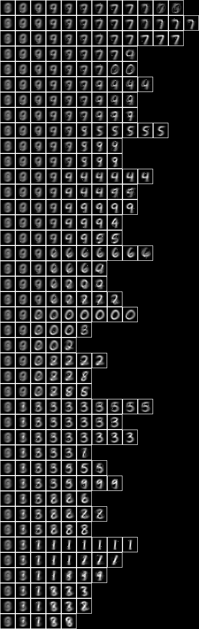
The larger model is correct for 70.0% of the test sample. The accuracy can be increased to 74.0% in a model consisting of a tree of 127 2-tuples, and to 75.5% in a model consisting of a tree of 511 1-tuples.
Now, instead of creating conditional entropy models directly on the pixel substrate, let us create them on an underlying level consisting of induced model derived variables. When we do this for the one level unsupervised model, above, we obtain a semi-supervised model,

This two level semi-supervised model has an accuracy of 77.3% which is higher than the 127 1-tuple conditional entropy model (70.0%) and the underlying unsupervised model (61.2%).
Repeating for the two level model, we obtain a different semi-supervised model,
This three level semi-supervised model has an accuracy of 77.8% which is also higher than the 127 1-tuple conditional entropy model (70.0%) and the underlying unsupervised model (61.0%).
Both of these semi-supervised models make more accurate predictions of digit than the non-induced Bayesian networks do, which suggests that there happens to be significant causal relations from some of the derived variables of the unsupervised models to digit.